Tidy text analysis of Brett Kavanaugh's testimony
Introduction and purpose
On Sept 27, 2018, an extraordinary hearing took place where the nominee for the Supreme Court Judge Brett Kavanaugh addressed questions from the Senate Judiciary Committee, as did his accuser Dr. Christine Ford. This text analysis is designed to uncover interesting patterns in how they spoke.
Libraries
We will use tidy methods to format and analyze the text. We load the tidy text analysis packages, as well as SnowballC to do basic word stemming later on (so that, for example, “beer” and “beers” are counted the same).
library(tidyverse)
library(tidytext)
library(SnowballC)
Committee names and party - for analysis by party later on.
names_party <- c(
  "GRASSLEY" = "Republican",
  "HATCH" = "Republican",
  "GRAHAM" = "Republican",
  "CORNYN" = "Republican",
  "LEE" = "Republican",
  "CRUZ" = "Republican",
  "FLAKE" = "Republican",
  "TILLIS" = "Republican",
  "SASSE" = "Republican",
  "CRAPO" = "Republican",
  "KENNEDY" = "Republican",
  "FEINSTEIN" = "Democrat",
  "LEAHY" = "Democrat",
  "WHITEHOUSE" = "Democrat",
  "KLOBUCHAR" = "Democrat",
  "COONS" = "Democrat",
  "BLUMENTHAL" = "Democrat",
  "HIRONO" = "Democrat",
  "BOOKER" = "Democrat",
  "HARRIS" = "Democrat",
  "MITCHELL" = "Nonpartisan",
  "FORD" = "Witness",
  "BROMWICH" = "Witness",
  "KAVANAUGH" = "Witness"
)
Load and preprocess data
The transcript was copied and pasted directly from a Washington Post story on Sept 29, 2018 and saved to a raw ASCII file transcript.txt. I copied only the part where the transcript of the hearing began (and skipped the introduction of the speakers). That text file is loaded into R and pre-processed here. I don’t include the transcript publicly because I don’t want to run into copyright issues, but I do load it using readLines with an encoding of UTF-8 into a character vector called trans_raw (not shown).
Preprocessing includes determining the speaker (in the Washington Post transcript, the speaker is given by last name in all caps, followed by a colon and space, and if a speaker speaks multiple lines the subsequent lines do not name the speaker). A regular expression is used to extract the speaker into a new column and then delete it from the text. The fill command is used for those subsequent lines where the speaker is implied. Some unhelpful lines are deleted from the transcript, including crosstalk and laughter where the “bag of words” philosophy is not helpful.
In addition to the preprocessing, I define a few new variables - the speaker number (a simple ordering of the speakers), the party of the speaker (defined by a mapping above), the last speaker and party (to, for example, examine sentiment or word usage in response to another speaker).
Finally, I convert the transcript into tidy format both with (_raw) and without U.S. English stop words.
n_lines <- length(trans_raw)

trans_df <- data_frame(raw = trans_raw) %>%
  mutate(line_number = row_number()) %>%
  slice(c(1:1310, 1342:n_lines)) %>% # you may have to tweak this
  mutate(is_ford = (row_number() < 1310), # you may have to tweak the line number here
         speaker = str_extract(raw, "^[\\(\\)\\?A-Z]{3,}")) %>%
  mutate(line = str_remove(raw, "^[\\(\\)\\?A-Z]+: ")) %>%
  fill(speaker) %>%
  mutate(last_speaker = lag(speaker, order_by = line_number)) %>%
  mutate(speaker_change = (line_number == 1 | speaker != lag(speaker, order_by = line_number)),
         speaker_number = cumsum(speaker_change)) %>%
  filter(!(str_detect(speaker, "CROSSTALK|CORRECTED|LAUGHTER|RECESS|GAVEL"))) %>%
  mutate(party = names_party[speaker]) %>%
  select(line_number, speaker_number, speaker, party, line)
## Warning: `data_frame()` is deprecated, use `tibble()`.
## This warning is displayed once per session.speakers_df <- trans_df %>%
group_by(speaker_number, speaker) %>%
slice(1) %>%
select(speaker_number, speaker) %>%
ungroup() %>%
filter(speaker != "(UNKNOWN)") %>%
mutate(last_speaker = lag(speaker),
last_speaker_party = names_party[last_speaker])
trans_df <- trans_df %>%
right_join(speakers_df) %>%
select(-line, line)## Joining, by = c("speaker_number", "speaker")trans_tidy_raw <- trans_df %>%
unnest_tokens(word, line)
trans_tidy <- trans_tidy_raw %>%
anti_join(stop_words)## Joining, by = "word"Word count
Here we count the number of words for each speaker.
trans_tidy_raw %>%
  group_by(speaker_number, speaker) %>%
  count() %>%
  ggplot(aes(x = speaker_number, y = n, group = speaker, color = speaker)) +
  geom_line() +
  scale_color_viridis_d()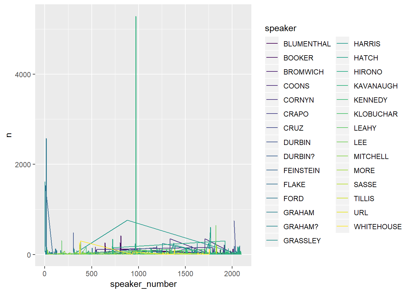
This isn’t too helpful. Grassley does have a lot of words, but that make sense because he is chairing the meeting.
Ford
It will be somewhat difficult to gauge Dr. Ford’s testimony by last speaker’s party, because the Republicans largely relied on a female sex crimes prosecutor to do their questioning.
trans_tidy %>%
  filter(speaker == "FORD") %>%
  inner_join(get_sentiments("bing")) %>%
  count(line_number, last_speaker_party, sentiment) %>%
  spread(sentiment, n, fill = 0) %>%
  mutate(sentiment = positive - negative) %>%
  ggplot(aes(x = line_number, y = sentiment)) +
  geom_line() +
  geom_hline(yintercept = 0, linetype = "dashed", color = gray(0.5)) +
  geom_point(aes(color = last_speaker_party)) +
  labs(x = "\"Time\" (as given by line number)", y = "Sentiment", color = "Last Speaker\nParty")
## Joining, by = "word"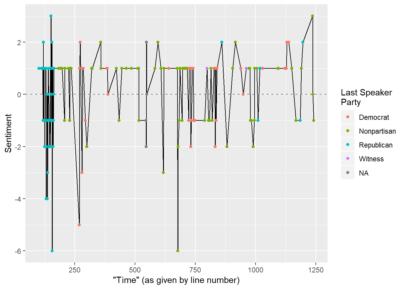
I’m not surprised that this analysis showed a lot of negative sentiment, but I am surprised that Dr. Ford for a large part kept her testimony within a tight window for sentiment. Notice the large amount of green - this indicates the last speaker was the “nonpartisan” staff counsel Rachel Mitchell.
Words in general
trans_tidy %>%
  filter(speaker == "FORD") %>%
  mutate(word = wordStem(word)) %>%
  count(word) %>%
  top_n(25, n) %>%
  ggplot(aes(fct_reorder(word,n))) +
  geom_bar(aes(weight = n)) +
  labs(x = "Stemmed word", y = "Times used in Ford's testimony") +
  coord_flip()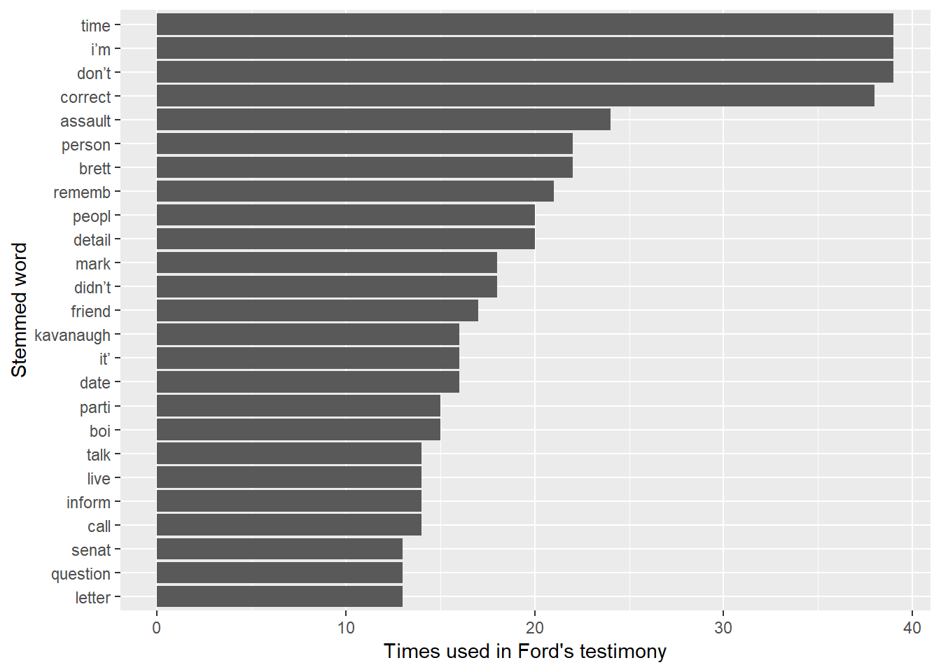
You can see several issues starting to emerge - “detail” is an important consideration as the #10 word, as well as words like “person”, “people”, “remember”, “mark”, and “assault”.
Words by party of last speaker
trans_tidy %>%
  filter(speaker == "FORD") %>%
  mutate(word = wordStem(word)) %>%
  count(word) %>%
  top_n(25, n) -> top_words

trans_tidy %>%
  filter(speaker == "FORD", !is.na(last_speaker_party)) %>%
  semi_join(top_words) %>% # semi-join is a filtering join - keep only top words above
  mutate(word = wordStem(word)) %>%
  count(last_speaker_party, word) %>%
  group_by(last_speaker_party) %>%
  mutate(ord = rank(n, ties.method = "random"),
         ord_word = paste0(sprintf("%03d",ord), "_", word)) %>% # needed for ordering within facet
  ungroup() %>%
  ggplot(aes(ord_word, n)) +
  geom_bar(stat = "identity") +
  labs(x = "Stemmed word", y = "Times used in Ford's testimony") +
  coord_flip() +
  facet_wrap(~ last_speaker_party, scales = "free") +
  scale_x_discrete(labels = function(x) str_remove(x,"^\\d+_"))
## Joining, by = "word"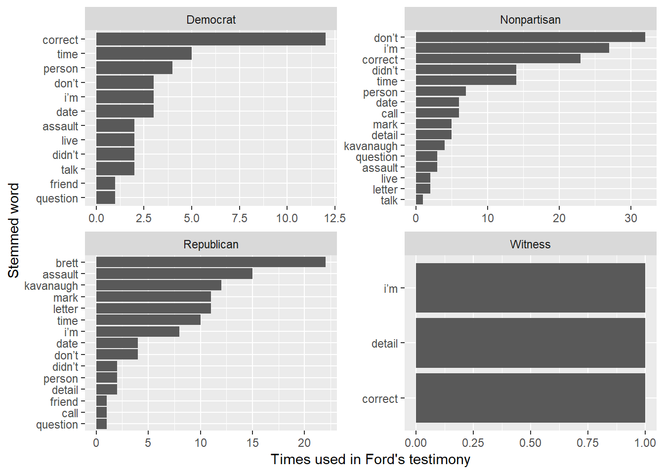
Here’s where we start to see quite a bit of difference in the language used to respond to the different parties. Dr. Ford used “detail” quite a bit after the staff counsel and Republicans but the word “correct” far and away the most often after the Democrats. There’s not a lot to gain from looking at the Witness facet in the graph, but do recall that indicates Dr. Ford’s lawyer.
Kavanaugh
Sentiment better after Republicans?
First, let’s get a word count after Democrats and Republicans
trans_tidy_raw %>%
  filter(speaker == "KAVANAUGH") %>%
  count(last_speaker_party)
## # A tibble: 5 x 2
## last_speaker_party n
## <chr> <int>
## 1 Democrat 4185
## 2 Nonpartisan 1334
## 3 Republican 6703
## 4 Witness 149
## 5 <NA> 508Not a lot too see here. I did not a lot of Republicans used their time to make their own statements about the hearing rather than ask questions (e.g. Lindsey Graham). Also, the count includes Judge Kavanaugh’s opening statment.
Now do a sentiment analysis after Democrats and Republicans.
trans_tidy %>%
  filter(speaker == "KAVANAUGH") %>%
  inner_join(get_sentiments("bing")) %>%
  count(last_speaker_party, sentiment) %>%
  spread(sentiment, n, fill = 0) %>%
  mutate(sentiment = positive - negative)
## Joining, by = "word"## # A tibble: 3 x 4
## last_speaker_party negative positive sentiment
## <chr> <dbl> <dbl> <dbl>
## 1 Democrat 66 25 -41
## 2 Nonpartisan 18 7 -11
## 3 Republican 143 104 -39Looks like he spoke negatively after each party, on average. This was expected, as he was under the gun.
Kavanaugh’s sentiment over time
Judge Kavanaugh was a sour and combative guy. Let’s see how he fared over time, with line_number as a surrogate for time.
trans_tidy %>%
  filter(speaker == "KAVANAUGH") %>%
  inner_join(get_sentiments("bing")) %>%
  count(line_number, last_speaker_party, sentiment) %>%
  spread(sentiment, n, fill = 0) %>%
  mutate(sentiment = positive - negative) %>%
  ggplot(aes(x = line_number, y = sentiment)) +
  geom_line() +
  geom_hline(yintercept = 0, linetype = "dashed", color = gray(0.5)) +
  geom_point(aes(color = last_speaker_party)) +
  labs(x = "\"Time\" (as given by line number)", y = "Sentiment", color = "Last Speaker\nParty")
## Joining, by = "word"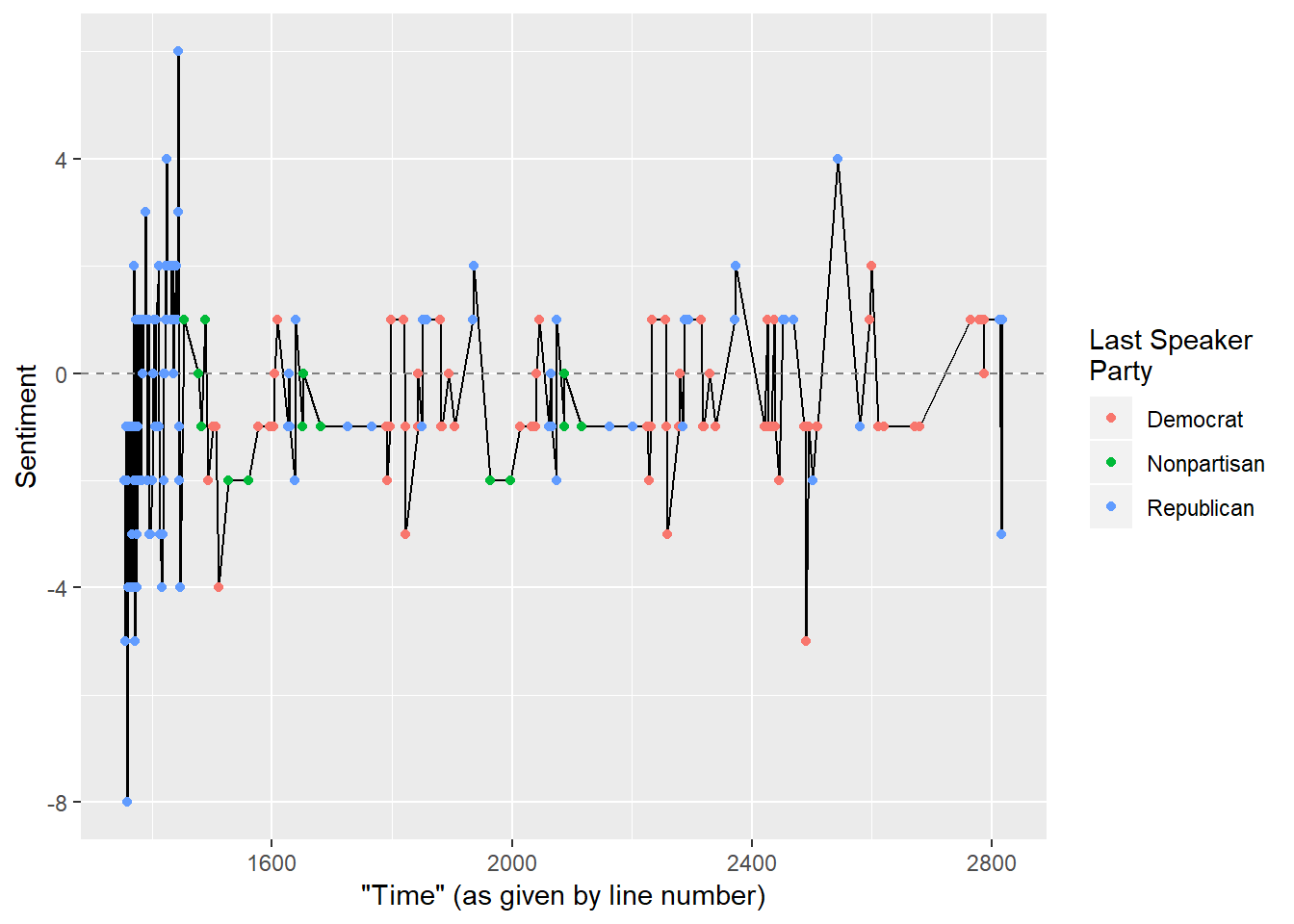
His opening statement (which included a lot of crying and angry statements) was on the balance negative, but he went all over the place. This is somewhat expected. During questioning, the sentiment content of words stayed within a tighter window for the most part.
Beer!
Let’s count the number of times he said beer, as this seemed to be an important part of the conversation.
trans_tidy %>%
  filter(speaker == "KAVANAUGH") %>%
  filter(word %in% c("beer", "beers")) %>% # maybe should add "ski" here
  count(last_speaker_party)
## # A tibble: 3 x 2
## last_speaker_party n
## <chr> <int>
## 1 Democrat 10
## 2 Nonpartisan 24
## 3 Republican 12One thing that is important, that will be missed by this rather cursory analysis for certain, is the use of rare words like “boof” and “Devil’s triangle”. The public has contested the meanings Kavanaugh gave in his testimony, and this transcript isn’t going to yield much more insight. There are also words such as “ski” that have various meanings. The Urban Dictionary may be helpful in those analyses, but math certainly won’t be.
Words in general
Here we will need to stem the words (so, for example, “beer” and “beers” are counted as the same word).
trans_tidy %>%
  filter(speaker == "KAVANAUGH") %>%
  mutate(word = wordStem(word)) %>%
  count(word) %>%
  top_n(25, n) %>%
  ggplot(aes(fct_reorder(word,n))) +
  geom_bar(aes(weight = n)) +
  labs(x = "Stemmed word", y = "Times used in Kavanaugh's testimony") +
  coord_flip()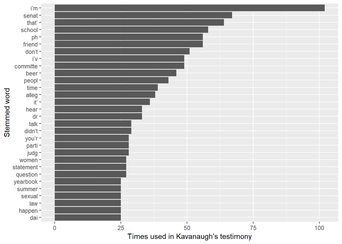
Our favorite word, beer, is Number 10. (“ph” appears to be an indicator in the transcript of some unintelligible or filler sounds, so he did that a lot).
Let’s see how he does in response to the different parties, but keep only the words above.
trans_tidy %>%
  filter(speaker == "KAVANAUGH") %>%
  mutate(word = wordStem(word)) %>%
  count(word) %>%
  top_n(25, n) -> top_words

trans_tidy %>%
  filter(speaker == "KAVANAUGH", !is.na(last_speaker_party)) %>%
  semi_join(top_words) %>% # semi-join is a filtering join - keep only top words above
  mutate(word = wordStem(word)) %>%
  count(last_speaker_party, word) %>%
  group_by(last_speaker_party) %>%
  mutate(ord = rank(n, ties.method = "random"),
         ord_word = paste0(sprintf("%03d",ord), "_", word)) %>% # needed for ordering within facet
  ungroup() %>%
  ggplot(aes(ord_word, n)) +
  geom_bar(stat = "identity") +
  labs(x = "Stemmed word", y = "Times used in Kavanaugh's testimony") +
  coord_flip() +
  facet_wrap(~ last_speaker_party, scales = "free") +
  scale_x_discrete(labels = function(x) str_remove(x,"^\\d+_"))
## Joining, by = "word"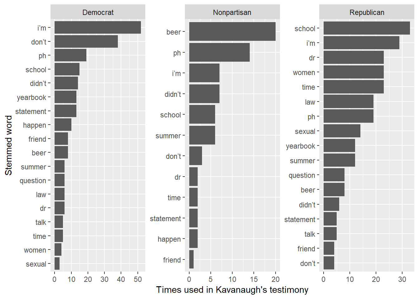
Nothing seems out of the ordinary for someone who is called to explain his beer consumption and attitudes/behavior toward women in school.
Conclusion
There are of course a lot of limitations to this approach, such as whether Judge Kavanaugh adequately addressed questions directed at him and the tone and nonverbal cues given by both witnesses. However, this cursory analysis has already yielded some interesting details about how the two different witnesses, and hopefully the data cleaning instructions and code at the top can help you with your own analysis.