Space launches (Tidy Tuesday Jan 15, 2019)
Purpose
This week’s Tidy Tuesday dataset, Space launches is also from The Economist. The article hypothesizes that the space race is dominated by “new contenders”. There are two data files, one describing space launch providers, and another describing individual launches. In this post I look at the number of launches by state, success, or both.
Setup and downloading data
agencies <- read_csv("https://raw.githubusercontent.com/rfordatascience/tidytuesday/master/data/2019/2019-01-15/agencies.csv")
launches <- read_csv("https://raw.githubusercontent.com/rfordatascience/tidytuesday/master/data/2019/2019-01-15/launches.csv")
Initial exploration
Data structure
This is what the agencies dataset looks like.
head(agencies) ## # A tibble: 6 x 19
## agency count ucode state_code type class tstart tstop short_name name
## <chr> <dbl> <chr> <chr> <chr> <chr> <chr> <chr> <chr> <chr>
## 1 RVSN 1528 RVSN SU O/LA D 1960 1991~ RVSN Rake~
## 2 UNKS 904 GUKOS SU O/LA D 1986 ~ 1991 UNKS Upra~
## 3 NASA 469 NASA US O/LA~ C 1958 ~ - NASA Nati~
## 4 USAF 388 USAF US O/LA~ D 1947 ~ - USAF Unit~
## 5 AE 258 AE F O/LA B 1980 ~ * Arianespa~ Aria~
## 6 AFSC 247 AFSC US LA D 1961 ~ 1992~ AFSC US A~
## # ... with 9 more variables: location <chr>, longitude <chr>,
## # latitude <chr>, error <chr>, parent <chr>, short_english_name <chr>,
## # english_name <chr>, unicode_name <chr>, agency_type <chr>This appears to be one dataset per agency that has participated in a launch.
My best guess for state codes:
- RU = Russia
- SU = Soviet Union
- US = United States
- F = France
- CN = China
- IN = India
- J = Japan
- I-ESA = European Space Agency
- IL = Israel
- I = Italy
- IR = Iran
- KP = North Korea
- CYM = Cayman Islands
- I-ELDO = Predecessor to ESA
- KR = Korea
- BR = Brazil
- UK = United Kingdom
Later on, we might combine SU and RU into one country, because the Soviet Union effectively changed into Russia for purposes here (I acknowledge the geopolitics is more complicated). The European Space Agency is a successor to the European Launch Development Organization, so it makes sense to combine I-ESA and I-ELDO as well.
And this is the launches dataset:
head(launches) ## # A tibble: 6 x 11
## tag JD launch_date launch_year type variant mission agency
## <chr> <dbl> <date> <dbl> <chr> <chr> <chr> <chr>
## 1 1967~ 2.44e6 1967-06-29 1967 Thor~ <NA> Secor ~ US
## 2 1967~ 2.44e6 1967-08-23 1967 Thor~ <NA> DAPP 3~ US
## 3 1967~ 2.44e6 1967-10-11 1967 Thor~ <NA> DAPP 4~ US
## 4 1968~ 2.44e6 1968-05-23 1968 Thor~ <NA> DAPP 5~ US
## 5 1968~ 2.44e6 1968-10-23 1968 Thor~ <NA> DAPP 6~ US
## 6 1969~ 2.44e6 1969-07-23 1969 Thor~ <NA> DAPP 7~ US
## # ... with 3 more variables: state_code <chr>, category <chr>,
## # agency_type <chr>This appears to be one dataset per launch.
Checking
Analysis of launches
By state
Number of launches by state:
launches %>%
  count(state_code, sort = TRUE)
## # A tibble: 17 x 2
## state_code n
## <chr> <int>
## 1 SU 2444
## 2 US 1716
## 3 RU 734
## 4 CN 302
## 5 F 291
## 6 J 115
## 7 IN 65
## 8 I-ESA 13
## 9 IL 10
## 10 I 9
## 11 IR 8
## 12 KP 5
## 13 CYM 4
## 14 I-ELDO 3
## 15 KR 3
## 16 BR 2
## 17 UK 2Launches by state and year:
launches %>%
  count(state_code, launch_year) %>%
  ggplot(aes(launch_year, n, group=state_code, color = state_code)) +
  geom_line() +
  labs(y = "Number of launches", x = "Year") +
  scale_color_discrete()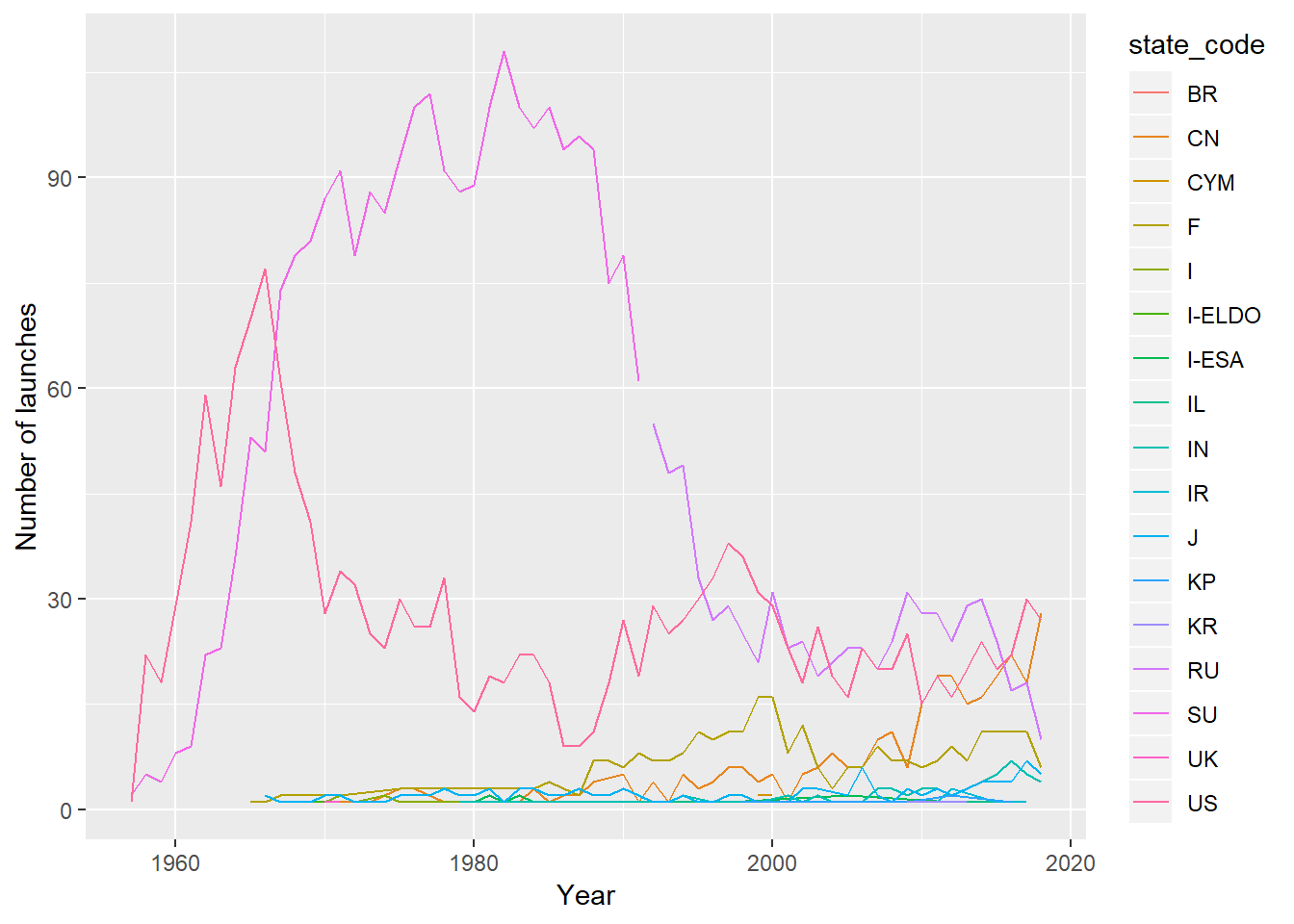
Observation: the Soviet Union and Russian programs appear to be a continuation of the same program, as evidenced by the break but same trend in the early 1990s between SU and RU. So in subsequent analyses we’ll combine SU and RU into RU.
Here we model the launches by state using a Poisson generalized linear model (GLM). In addition to the Russia combining, I combine European State Agency and ELDO, which are also continuations of the same agency, more or less.
launches %>%
  mutate(state_code = ifelse(state_code == "SU", "RU", state_code),
         state_code = ifelse(state_code %in% c("I-ESA", "I-ELDO"), "EU", state_code),
         launch_year_norm = launch_year - 1957) %>%
  count(launch_year_norm, state_code) %>%
  filter(state_code %in% c("US", "RU", "CN", "EU", "J")) %>%
  ungroup() ->
  launch_stcl

newdat <- crossing(launch_year_norm = unique(launch_stcl$launch_year_norm),
                   state_code = unique(launch_stcl$state_code))

launch_stcl %>%
  glm(n ~ launch_year_norm * state_code, family = "poisson", data = .) ->
  mod

mod %>%
  augment(newdata = newdat, type.predict = "response") %>%
  mutate(launch_year = launch_year_norm + 1957) %>%
  ggplot(aes(launch_year, .fitted, group = state_code, color = state_code)) +
  geom_line() +
  labs(y = "Fitted number of launches", x = "Launch year", color = "State")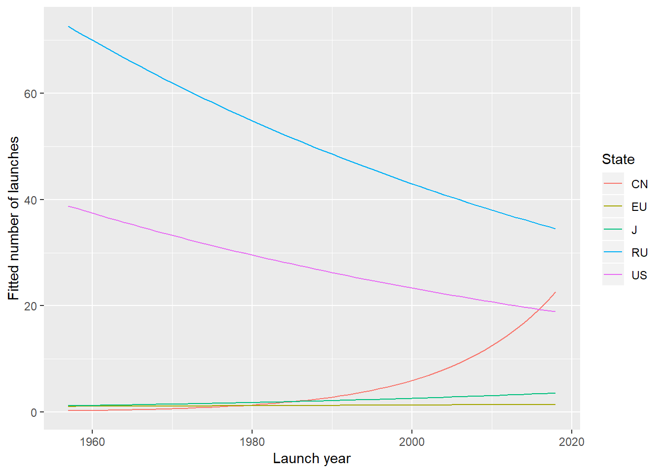
Doesn’t really give a lot (and again, modeled values have to be treated with a grain of salt but are otherwise ok for suggesting trends), but the US and Soviet Union did a lot of launches in the 60s-70s while other countries only dabbled their toes.
Private or startup vs. state
Here we calculate the overall percentage of state-sponsored launches (as opposed to commercial launches)by year and graph. We combine “private” and “startup” into one group for now.
launches %>%
  mutate(is_state = ifelse(agency_type == "state", "Yes", "No")) %>%
  count(launch_year, is_state) %>%
  group_by(launch_year) %>%
  mutate(percentage = n / sum(n)) %>%
  filter(is_state == "Yes") %>%
  ggplot(aes(launch_year, percentage)) +
  geom_line() +
  geom_point() +
  expand_limits(y = c(0, NA)) +
  scale_y_continuous(labels = scales::percent_format()) +
  labs(y = "Launched by state", x = "Launch year", color = "State")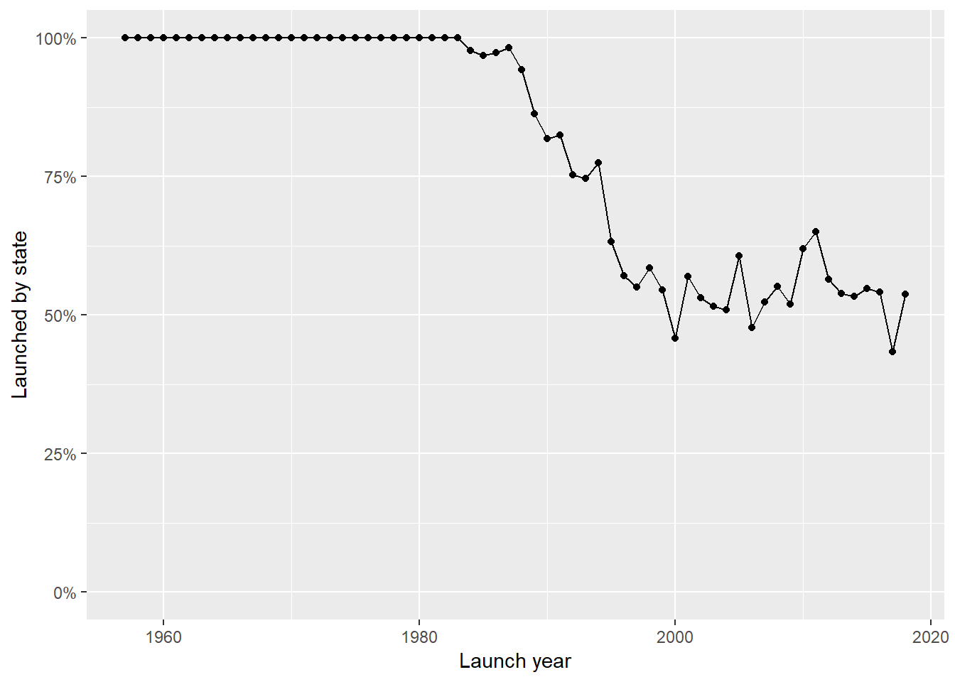
As The Economist noted, private launches really didn’t start until after the Challenger explosion in 1986. Since then, commercial enterprises have been pushing more into the space launch space.
Private vs. startup vs. state
Here we look at all three categories. In addition, we use an area graph because we are showing relative percentages.
launches %>%
  count(launch_year, agency_type) %>%
  group_by(launch_year) %>%
  mutate(percentage = n / sum(n)) %>%
  ggplot(aes(launch_year, percentage, group = agency_type, fill = agency_type)) +
  geom_area() +
  expand_limits(y = c(0, NA)) +
  scale_y_continuous(labels = scales::percent_format()) +
  labs(x = "Launch year", y = "Percentages of launches", fill = "Agency type")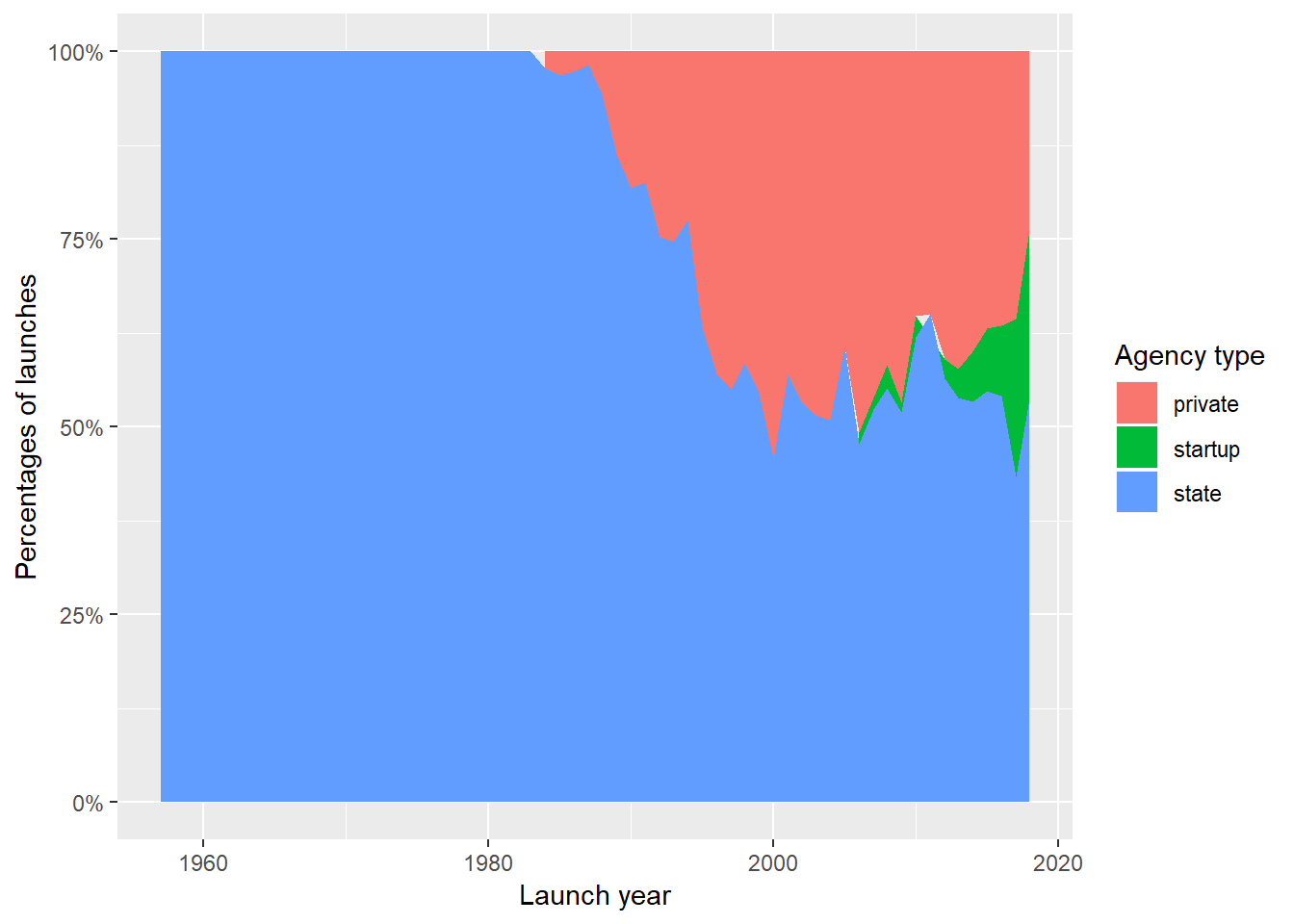
The startup phenomenon is fairly recent, but has really taken off. (Pun intended.)
Whether it is worth exploring startups further depends on where they are:
launches %>%
  mutate(state_code = ifelse(state_code == "SU", "RU", state_code),
         state_code = ifelse(state_code %in% c("I-ESA", "I-ELDO"), "EU", state_code)) %>%
  filter(agency_type == "startup")
## # A tibble: 70 x 11
## tag JD launch_date launch_year type variant mission agency
## <chr> <dbl> <date> <dbl> <chr> <chr> <chr> <chr>
## 1 2018~ 2.46e6 2018-01-21 2018 Elec~ <NA> Dove/L~ RLABU
## 2 2017~ 2.46e6 2017-05-25 2017 Elec~ <NA> <NA> RLABU
## 3 2008~ 2.45e6 2008-09-28 2008 Falc~ <NA> Mass s~ SPX
## 4 2009~ 2.46e6 2009-07-14 2009 Falc~ <NA> MACSat SPX
## 5 2010~ 2.46e6 2010-06-04 2010 Falc~ <NA> Dragon~ SPX
## 6 2010~ 2.46e6 2010-12-08 2010 Falc~ <NA> Dragon~ SPX
## 7 2012~ 2.46e6 2012-05-22 2012 Falc~ <NA> Dragon~ SPX
## 8 2012~ 2.46e6 2012-10-08 2012 Falc~ <NA> Dragon~ SPX
## 9 2013~ 2.46e6 2013-03-01 2013 Falc~ <NA> Dragon~ SPX
## 10 2013~ 2.46e6 2013-09-29 2013 Falc~ 1.1 Cassio~ SPX
## # ... with 60 more rows, and 3 more variables: state_code <chr>,
## # category <chr>, agency_type <chr>These are all in the US, so when we analyze startup trends later we’ll have to look at the US only and restrict interpretation. The number of startup launches per year is as follows:
launches %>%
  mutate(state_code = ifelse(state_code == "SU", "RU", state_code),
         state_code = ifelse(state_code %in% c("I-ESA", "I-ELDO"), "EU", state_code)) %>%
  filter(agency_type == "startup") %>%
  count(launch_year) %>%
kable()| launch_year | n |
|---|---|
| 2006 | 1 |
| 2007 | 1 |
| 2008 | 2 |
| 2009 | 1 |
| 2010 | 2 |
| 2012 | 2 |
| 2013 | 3 |
| 2014 | 6 |
| 2015 | 7 |
| 2016 | 8 |
| 2017 | 19 |
| 2018 | 18 |
Private vs. state by state
Some data manipulation here. We again group private and startup launches and compare to state launches (and count startups as part of the private sector).
launches %>%
  mutate(is_state = ifelse(agency_type == "state", "Yes", "No"),
         state_code = ifelse(state_code == "SU", "RU", state_code),
         state_code = ifelse(state_code %in% c("I-ESA", "I-ELDO"), "EU", state_code)) %>%
  count(launch_year, state_code, is_state) %>%
  group_by(launch_year, state_code) %>%
  mutate(percentage = n / sum(n)) %>%
  ungroup() %>%
  filter(is_state == "Yes", state_code %in% c("US", "RU", "J", "EU")) %>%
  ggplot(aes(launch_year, percentage, group = state_code, color = state_code)) +
  geom_line() + expand_limits(y = c(0, NA)) +
  scale_y_continuous(labels = scales::percent_format()) +
  labs(y = "Launched by state", x = "Launch year", color = "State")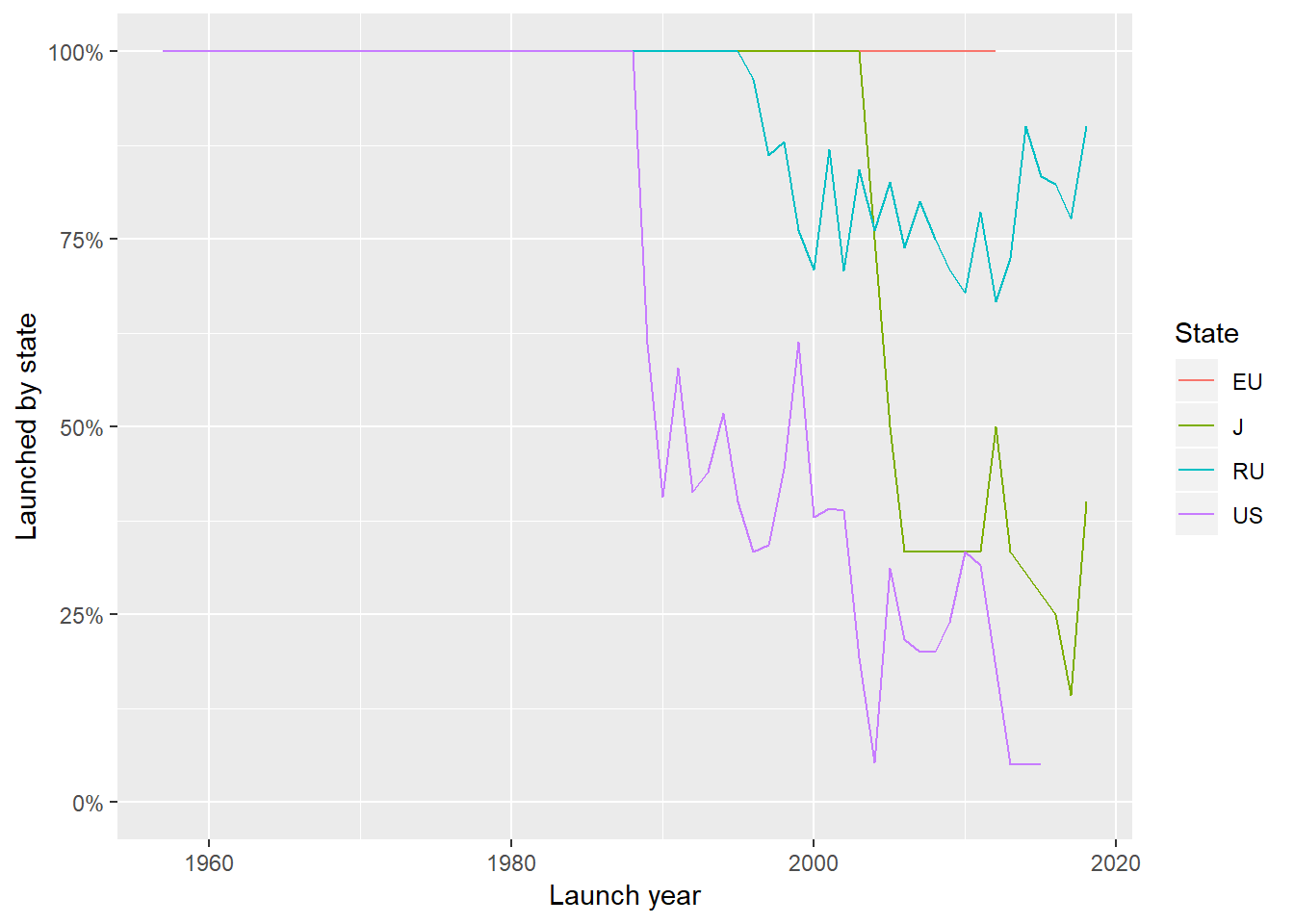
I played around with this a bit, and it looks like all other states use exclusively state-sponsored launches.
launches %>%
  mutate(is_state = ifelse(agency_type == "state", "Yes", "No"),
         state_code = ifelse(state_code == "SU", "RU", state_code),
         state_code = ifelse(state_code %in% c("I-ESA", "I-ELDO"), "EU", state_code)) %>%
  filter(state_code %in% c("US", "RU", "EU", "J", "CN", "IN")) ->
  launches_state

newdat <- crossing(launch_year = unique(launches_state$launch_year),
                   state_code = unique(launches_state$state_code))

launches_state %>%
  glm(agency_type == "state" ~ launch_year * state_code, family = "binomial", data = .) ->
  mod

mod %>%
  augment(newdata = newdat, type.predict = "response") %>%
  ggplot(aes(launch_year, .fitted, group = state_code, color = state_code)) +
  geom_line() +
  scale_y_continuous(labels = scales::percent_format(accuracy = 1)) +
  labs(y = "Probability of state launch", x = "Launch year", color = "State")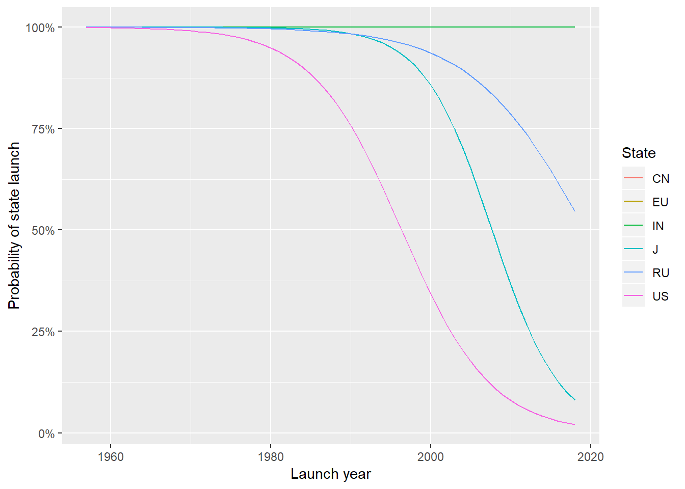
While you’ll have to take the modeled values with a grain of salt, it is interesting to see the trends for each state. The US and Japan are increasing reliance on commercial launches, and Russia is starting to as well. Other countries rely exclusively on state launches.
Launch success
The following is the overall launch success.
launches %>%
  count(launch_year, category) %>%
  group_by(launch_year) %>%
  mutate(percentage = n / sum(n)) %>%
  filter(category == "O") %>%
  ggplot(aes(launch_year, percentage)) +
  geom_line() + expand_limits(y = c(0, NA)) +
  scale_y_continuous(labels = scales::percent_format()) +
  labs(y = "Success rate", x = "Launch year")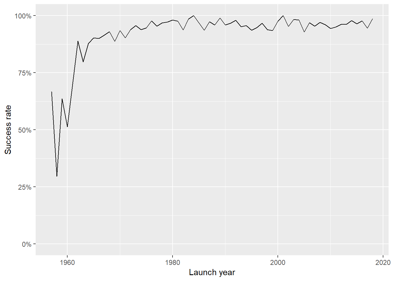
The 1950s and 1960s were a time for developing technology. By 1969 we had put a man on the moon. We kept refining the technology to have a high launch success rate (high-profile failures, such as the Challenger, notwithstanding).
Launch success by state
Here we look at each state’s journey to perfect space launch technology, at least through the singular metric of launch success. This is a bit noisy, and a lot of countries only have a few launches.
launches %>%
  mutate(is_state = ifelse(agency_type == "state", "Yes", "No"),
         state_code = ifelse(state_code == "SU", "RU", state_code),
         state_code = ifelse(state_code %in% c("I-ESA", "I-ELDO"), "EU", state_code)) %>%
  count(launch_year, state_code, category) %>%
  group_by(launch_year, state_code) %>%
  mutate(percentage = n / sum(n)) %>%
  ungroup() %>%
  filter(category == "O", state_code %in% c("US", "RU", "EU", "J", "CN", "IN")) %>%
  # filter(category == "O", state_code %in% c("EU")) %>%
  ggplot(aes(launch_year, percentage, group = state_code, color = state_code)) +
  geom_line() + expand_limits(y = c(0, NA)) +
  scale_y_continuous(labels = scales::percent_format()) +
  labs(y = "Launch success", x = "Launch year", color = "State")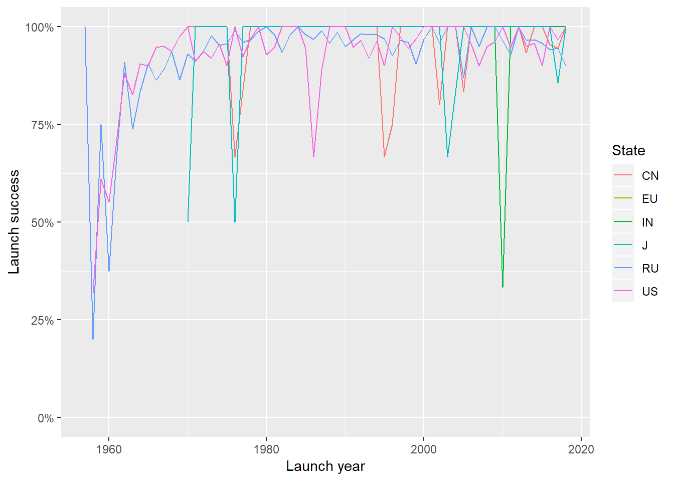
Most years after 1970 showed high success rates, with “off” years for some states (which probably had few launches). We model this to try to tease out some signal or trend from the noise:
launches %>%
  mutate(is_state = ifelse(agency_type == "state", "Yes", "No"),
         state_code = ifelse(state_code == "SU", "RU", state_code),
         state_code = ifelse(state_code %in% c("I-ESA", "I-ELDO"), "EU", state_code)) %>%
  filter(state_code %in% c("US", "RU", "EU", "J", "CN", "IN")) ->
  launches_success

newdat <- crossing(launch_year = unique(launches_success$launch_year),
                   state_code = unique(launches_success$state_code))

launches_success %>%
  glm(category == "O" ~ launch_year * state_code, family = "binomial", data = .) ->
  mod

mod %>%
  augment(newdata = newdat, type.predict = "response") %>%
  ggplot(aes(launch_year, .fitted, group = state_code, color = state_code)) +
  geom_line() +
  scale_y_continuous(labels = scales::percent_format(accuracy = 1)) +
  labs(y = "Probability of successful launch", x = "Launch year", color = "State") +
  labs(caption = "Note: model for IN and EU is suspect")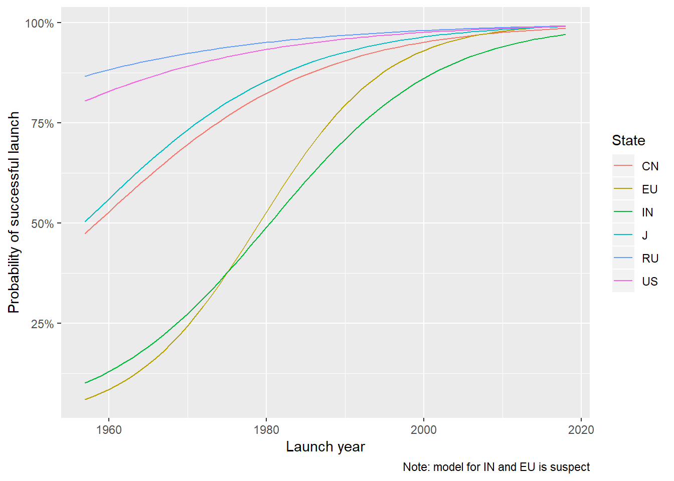
So, before, say, 1970, it only makes sense for Russia and the US to have success rates. The trend lines for India and the EU are suspect. (I think India was dragged down by an outlier, and the model wasn’t very good for the EU due to the consistently high success rates. In addition, the data isn’t very robust for these two states.) Always compare the fitted or smoothed graphs to the raw. I added a caveat into the visualization.
Launch agencies in the US
Because the US is starting to rely on startups, it is worth exploring success rates by agency. We start with the agencies themselves.
launches %>%
  mutate(is_state = ifelse(agency_type == "state", "Yes", "No")) %>%
  filter(state_code == "US") %>%
  count(launch_year, agency) %>%
  left_join(agencies %>% select(agency,name) %>% bind_rows(tibble(agency = "US", name = "US"))) %>%
  mutate(name = if_else(str_detect(name, "Boeing"), "Boeing", name),
         name = if_else(str_detect(name, "Lockheed"), "Lockheed", name),
         name = if_else(str_detect(name, "Orbital"), "Orbital", name),
         name = if_else(str_detect(name, "Martin Marietta"), "Martin Marietta", name),
         name = if_else(str_detect(name, "McDonnell Douglas"), "McDonnell Douglas", name),
         name = if_else(str_detect(name, "General Dynamics"), "General Dynamics", name),
         name = str_sub(name,1,10)) %>%
  group_by(launch_year) %>%
  mutate(percentage = n / sum(n)) %>%
  ungroup() %>%
  ggplot(aes(launch_year, percentage, group = name, fill = name)) +
  geom_area() + expand_limits(y = c(0, NA)) +
  scale_y_continuous(labels = scales::percent_format()) +
  scale_fill_viridis_d() +
  labs(y = "Percentage of launches", x = "Launch year", fill = "Agency")
## Joining, by = "agency"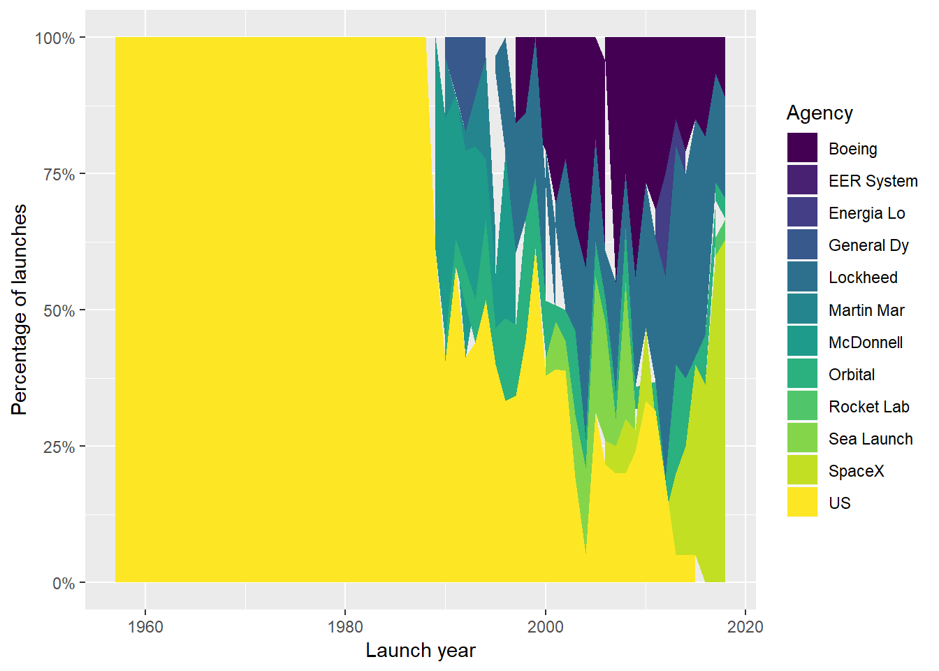
To try to cut down on noise, I tried to combine similar agencies, and finally cut the names short because that little bit of ugliness was preferable to a squished graph. A couple of things jump out:
- The US launches have basically gone to 0
- Boeing and Lockheed have been mainstays in the space launch area since the late 80s
- SpaceX has really been aggressive in space launches in the last couple of years (no surprise)
Now, for how successful they are:
launches %>%
  mutate(is_state = ifelse(agency_type == "state", "Yes", "No")) %>%
  filter(state_code == "US") %>%
  left_join(agencies %>% select(agency,name) %>% bind_rows(tibble(agency = "US", name = "US"))) %>%
  mutate(name = if_else(str_detect(name, "Boeing"), "Boeing", name),
         name = if_else(str_detect(name, "Lockheed"), "Lockheed", name),
         name = if_else(str_detect(name, "Orbital"), "Orbital", name),
         name = if_else(str_detect(name, "Martin Marietta"), "Martin Marietta", name),
         name = if_else(str_detect(name, "McDonnell Douglas"), "McDonnell Douglas", name),
         name = if_else(str_detect(name, "General Dynamics"), "General Dynamics", name),
         name = str_sub(name,1,10)) %>%
  count(launch_year, name, category) %>%
  group_by(launch_year, name) %>%
  mutate(percentage = n / sum(n)) %>%
  ungroup() %>%
  filter(category == "O") %>%
  ggplot(aes(launch_year, percentage, group = name, color = name)) +
  geom_line() + expand_limits(y = c(0, NA)) +
  scale_y_continuous(labels = scales::percent_format()) +
  scale_color_viridis_d() +
  labs(y = "Launch success", x = "Launch year", color = "Agency")
## Joining, by = "agency"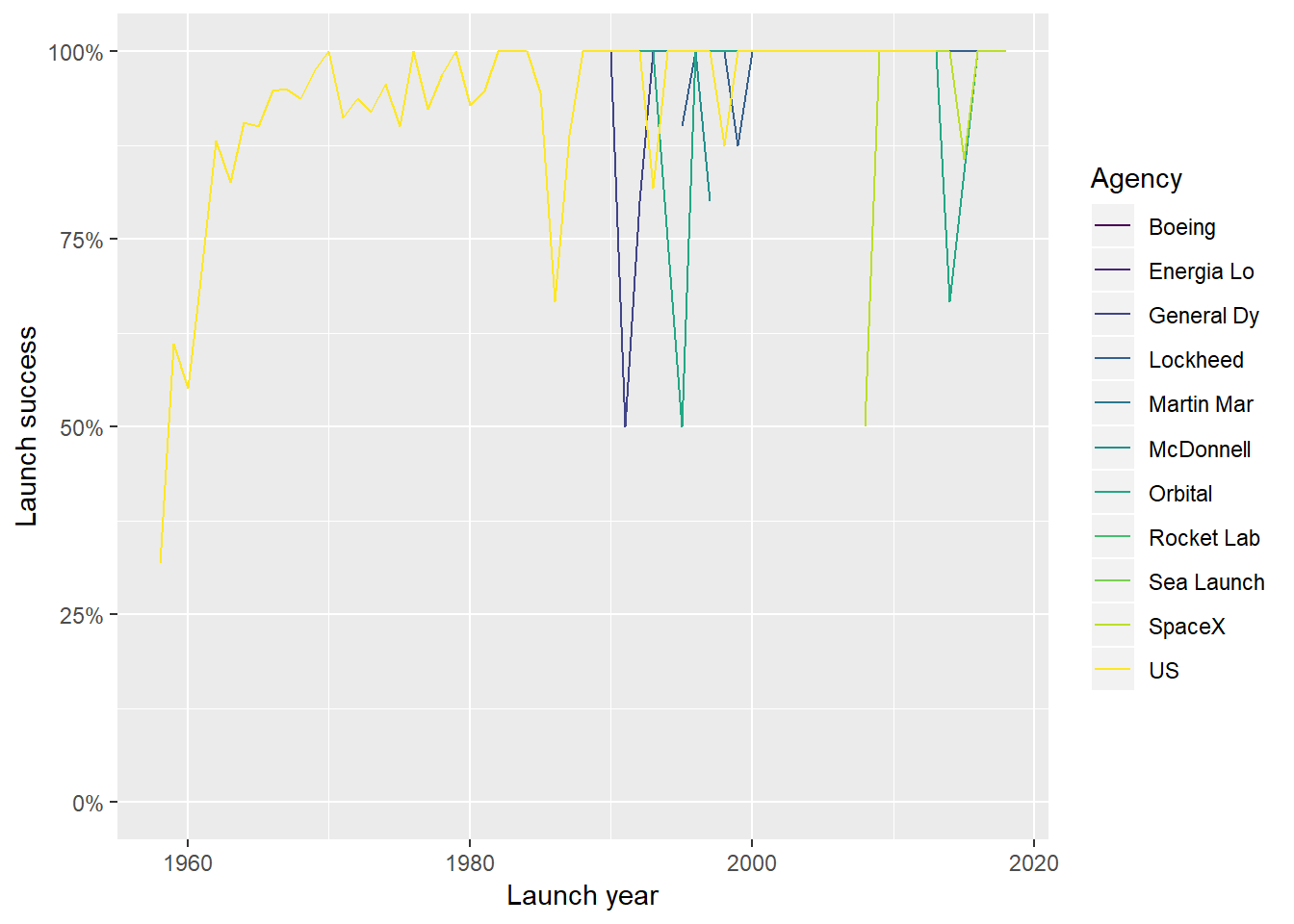
Most agencies have had a high success rate, with the exception of the US before 1965 or 1970 (perfecting technology), Boeing and Lockheed early on, and the odd years when startups are trying new things. It’s probably not worth trying to smooth these out or model them, because the data are getting sparse.
One word of warning. I don’t think the agencies dataset is entirely complete. This is data on what can be clandestine activities. Take this analysis with a grain of salt.
Discussion
It’s clear that the space race is dominated in the US by “new contenders”. This is especially true of the startups. There are also trends in Japan and Russia towards use of commercial launches, though not by startups. Old commercial mainstays, such as Boeing, remain in the launch business. Success in space launches has been high since the 1970s or even late 1960s, with a few exceptions. Some recent launch failures may be attributable to attempts at innovation in launch technology.