Reparameterizing models with Stan
Purpose
In the previous post, we took advantage of the rich structure of the Greenville flight data, especially the notions that the number of flights could depend on the weekday and the season of the flights. However, when we put the two together in what seemed like a natural way, we noticed that we started getting convergence problems, and if you looked carefully at the output, you would have noticed something very strange about the weekday estimates - they were all negative! As it turns out, this model is overdetermined - there are too many parameters. Thus, there could be an infinite number of solutions to this problem. I had glossed over this idea when I added only quarters to the model, but adding both we have to face it head on. We do that here.
Setup and data
library(tidyverse)
library(lubridate)
library(rstan)
library(bayesplot)
load("airline_data.RData")
airline_data %>%
  mutate(date=ymd(YEAR*10000+MONTH*100+DAY_OF_MONTH),
         wnum = floor((date - ymd(YEAR*10000+0101))/7)) ->
  airline_data

airline_data %>%
  filter(ORIGIN_AIRPORT_ID==11996) %>%
  count(date) ->
  counts_depart
options(mc.cores = parallel::detectCores())
rstan_options(auto_write = TRUE)Reparameterizing
Right now we have a model that looks like the following:
\[flights = q_i + w_j + \epsilon \left(i\in \left\{1,2,3,4\right\}, j\in\left\{1,2,3,4,5,6,7\right\}\right)\],
where \(\epsilon \sim \mathscr{N}\left(0,\sigma^2\right)\). This has an infinite number of solutions. For example, we can find a solution, then subtract 100 from all the \(w_j\) and add 100 to the \(q_i\) and still have a valid solution. Stan found one of them, but it started looking like there was a bit of trouble, and having all the \(w_j\) be negative doesn’t seem to be helpful for interpretation. Instead, let’s pick a model that will have a single solution. First, let’s go back to an overall mean concept. Then we will add in constraints that the sum of the quarter effects is 0, and as well the sum of the weekday effects is 0. This then should be completely determined and have a unique solution (we call this “identifiable” in the statistical modeling world). In math symbols, it looks like this:
\[flights = \mu + q_i + w_j + \epsilon \left(i\in \left\{1,2,3,4\right\}, j\in\left\{1,2,3,4,5,6,7\right\},\sum_{i=1}^4q_i=0,\sum_{j=1}^7w_j=0\right)\]
Let’s see what this looks like in Stan:
data {
  int ndates;
  vector[ndates] flights;
  int qtr[ndates];
  int dow[ndates];
}

parameters {
  real mu;
  real<lower=0> sigma;
  vector[3] qtr_effect_raw;
  vector[6] dow_effect_raw;
}

transformed parameters {
  vector[4] qtr_effect;
  for (i in 1:3)
    qtr_effect[i] = qtr_effect_raw[i];
  qtr_effect[4] = -sum(qtr_effect);

  vector[7] dow_effect;
  for (j in 1:6)
    dow_effect[j] = dow_effect_raw[j];
  dow_effect[7] = -sum(dow_effect);
}

model {
  flights ~ normal(mu + qtr_effect[qtr] + dow_effect[dow],sigma);
  sigma ~ uniform(0,20);
  mu ~ normal(32,10);
  for (i in 1:3)
    qtr_effect_raw[i] ~ normal(0,10);
  for (j in 1:6)
    dow_effect_raw[j] ~ normal(0,10);
}
Here, we use the transformed parameters block to enforce our idea that the sums of the quarter effects and the day of week effects are 0. If you look at what we did in that block, we basically set \(q_4 = -(q_1 + q_2 + q_3)\) and similarly for \(w_7\).
Now, how did I come up with this bit of wizardry? Stan is supposed to be be intuitive! Well, much of it is. And the use of transformed parameters states very clearly what is going on. How I came up with this bit of sorcery is by reading the Stan documentation, specifically Page 135 on identifiabilty.
The lovely part of this? The R code is the same as before, with the exception that I’m changing the variable name of the fit object.
ndates <- nrow(counts_depart)
flights <- counts_depart$n
qtr <- quarter(counts_depart$date)
dow <- wday(counts_depart$date)

data_to_pass <- c("ndates","flights","qtr","dow")
qtr_dow_model_reparm_fit <- stan("flights_qtr_dow_reparm.stan",data=data_to_pass)
## DIAGNOSTIC(S) FROM PARSER:
## Info (non-fatal):
## Left-hand side of sampling statement (~) may contain a non-linear transform of a parameter or local variable.
## If it does, you need to include a target += statement with the log absolute determinant of the Jacobian of the transform.
## Left-hand-side of sampling statement:
## qtr_effect[i] ~ normal(...)
## Info (non-fatal):
## Left-hand side of sampling statement (~) may contain a non-linear transform of a parameter or local variable.
## If it does, you need to include a target += statement with the log absolute determinant of the Jacobian of the transform.
## Left-hand-side of sampling statement:
## dow_effect[i] ~ normal(...)save(qtr_dow_model_reparm_fit,file="qtr_dow_model_reparm_fit.RData")
qtr_dow_model_reparm_fit## Inference for Stan model: flights_qtr_dow_reparm.
## 4 chains, each with iter=2000; warmup=1000; thin=1;
## post-warmup draws per chain=1000, total post-warmup draws=4000.
##
## mean se_mean sd 2.5% 25% 50% 75%
## mu 17.35 0.00 0.13 17.10 17.26 17.35 17.44
## sigma 2.28 0.00 0.09 2.12 2.22 2.28 2.34
## qtr_effect_raw[1] -3.52 0.00 0.22 -3.94 -3.66 -3.52 -3.37
## qtr_effect_raw[2] 2.87 0.00 0.21 2.45 2.72 2.87 3.01
## qtr_effect_raw[3] 0.41 0.00 0.24 -0.07 0.25 0.42 0.57
## dow_effect_raw[1] -0.83 0.00 0.30 -1.44 -1.03 -0.83 -0.63
## dow_effect_raw[2] 0.87 0.00 0.31 0.28 0.67 0.87 1.08
## dow_effect_raw[3] 0.92 0.00 0.30 0.33 0.71 0.92 1.12
## dow_effect_raw[4] 1.46 0.00 0.30 0.88 1.25 1.45 1.66
## dow_effect_raw[5] 1.40 0.00 0.30 0.79 1.19 1.40 1.60
## dow_effect_raw[6] 1.13 0.00 0.32 0.51 0.91 1.12 1.34
## qtr_effect[1] -3.52 0.00 0.22 -3.94 -3.66 -3.52 -3.37
## qtr_effect[2] 2.87 0.00 0.21 2.45 2.72 2.87 3.01
## qtr_effect[3] 0.41 0.00 0.24 -0.07 0.25 0.42 0.57
## qtr_effect[4] 0.24 0.00 0.21 -0.19 0.10 0.24 0.38
## dow_effect[1] -0.83 0.00 0.30 -1.44 -1.03 -0.83 -0.63
## dow_effect[2] 0.87 0.00 0.31 0.28 0.67 0.87 1.08
## dow_effect[3] 0.92 0.00 0.30 0.33 0.71 0.92 1.12
## dow_effect[4] 1.46 0.00 0.30 0.88 1.25 1.45 1.66
## dow_effect[5] 1.40 0.00 0.30 0.79 1.19 1.40 1.60
## dow_effect[6] 1.13 0.00 0.32 0.51 0.91 1.12 1.34
## dow_effect[7] -4.94 0.00 0.30 -5.52 -5.14 -4.94 -4.73
## lp__ -444.11 0.05 2.40 -449.81 -445.48 -443.77 -442.35
## 97.5% n_eff Rhat
## mu 17.60 5119 1
## sigma 2.47 5407 1
## qtr_effect_raw[1] -3.09 5162 1
## qtr_effect_raw[2] 3.29 4892 1
## qtr_effect_raw[3] 0.88 4421 1
## dow_effect_raw[1] -0.25 4796 1
## dow_effect_raw[2] 1.49 5070 1
## dow_effect_raw[3] 1.51 4582 1
## dow_effect_raw[4] 2.04 4492 1
## dow_effect_raw[5] 2.00 5009 1
## dow_effect_raw[6] 1.74 4852 1
## qtr_effect[1] -3.09 5162 1
## qtr_effect[2] 3.29 4892 1
## qtr_effect[3] 0.88 4421 1
## qtr_effect[4] 0.64 5829 1
## dow_effect[1] -0.25 4796 1
## dow_effect[2] 1.49 5070 1
## dow_effect[3] 1.51 4582 1
## dow_effect[4] 2.04 4492 1
## dow_effect[5] 2.00 5009 1
## dow_effect[6] 1.74 4852 1
## dow_effect[7] -4.34 4450 1
## lp__ -440.48 2081 1
##
## Samples were drawn using NUTS(diag_e) at Tue Jan 08 16:28:17 2019.
## For each parameter, n_eff is a crude measure of effective sample size,
## and Rhat is the potential scale reduction factor on split chains (at
## convergence, Rhat=1).So if you look at the messages from the compiling, you get the following:
DIAGNOSTIC(S) FROM PARSER:
Warning (non-fatal):
Left-hand side of sampling statement (~) may contain a non-linear transform of a parameter or local variable.
If it does, you need to include a target += statement with the log absolute determinant of the Jacobian of the transform.
Left-hand-side of sampling statement:
    qtr_effect[i] ~ normal(...)
Things just got real! Stan was warning us that we would have to start doing things by hand! Fortunately, we can ignore that for now But as you start adding in fancier nonlinear transforms, you will have to start paying attention to this. We’re far away from that in this series.
Let’s look at the convergence diagnostics. All the Rhats are 1, and the n_effs are close to or equal to 4000. So far so good, and it looks like our reparameterization is working. Let’s look at the traceplot of the quarter effects:
p <- mcmc_trace(as.array(qtr_dow_model_reparm_fit),pars="sigma",regex_pars = "qtr_effect\\[",
                facet_args = list(nrow = 5, labeller = label_parsed))
p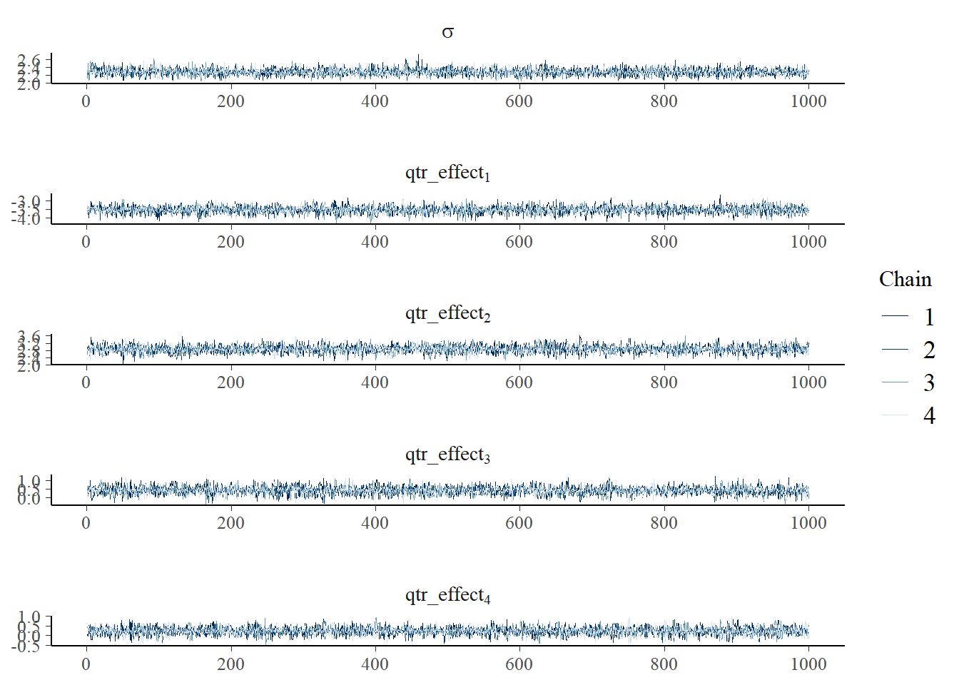
Nothing looks concerning here. I leave it up to you to look at the same for the day of week effects. Let’s look at the density plot of the overall effects \(\mu\) and \(\sigma\):
p <- mcmc_areas(as.matrix(qtr_dow_model_reparm_fit),pars=c("mu","sigma"),prob = 0.5) +
  ggtitle("Posterior distributions with medians and 50% intervals")
p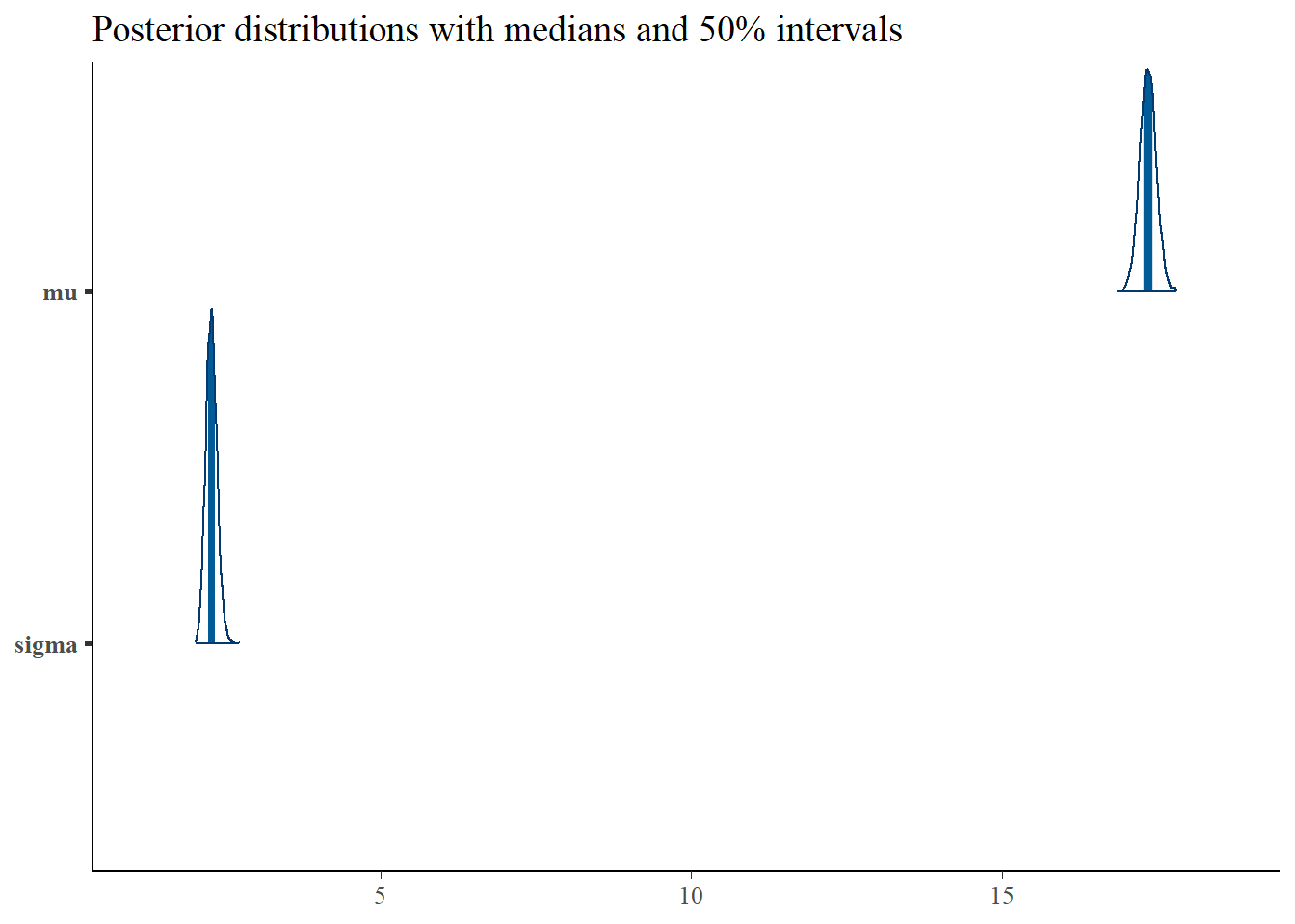
\(\mu\) here close to what we had in the mean model. However, \(\sigma\) is about half the magnitude, indicating that we have successfully explained a large part of the variance in number of flights using the quarter and day of week.
Now let’s look at the density plots of the quarter effects:
p <- mcmc_areas(as.matrix(qtr_dow_model_reparm_fit),regex_pars = "qtr_effect\\[",prob = 0.5) +
  ggtitle("Posterior distributions with medians and 50% intervals")
p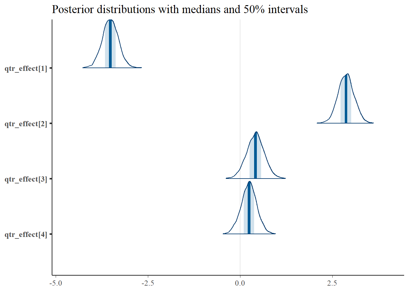
So, we can interpret this plot as Quarter 2 as the busiest quarters, which makes sense because Quarter 2 is the season of summer vacations. Also, in the original line plot, we noticed that the airport has the most departing flights in the summer, and that comes through here. Quarter 1 is by far the slowest.
There was a trick with the regex_pars that I used. I used regex_pars = "qtr_effect\\[" rather than regex_pars = "qtr_effect" because I wanted to exclude the redundant qtr_effect_raw variables. They were just temporary tools that we used to get qtr_effect to behave the way we wanted, but we really don’t want to perform inference on them. R has a few oddities in the way you use regular expressions, including the use of the double backslash \\ in certain situations. Here I wanted to force Stan to show only those qtr_effect variables followed directly by the character [ indicating an index number. The same trick applies to dow_effect below as well.
Here are the density plots of the weekday effects.
p <- mcmc_areas(as.matrix(qtr_dow_model_reparm_fit),regex_pars = "dow_effect\\[",prob = 0.5) +
  ggtitle("Posterior distributions with medians and 50% intervals")
p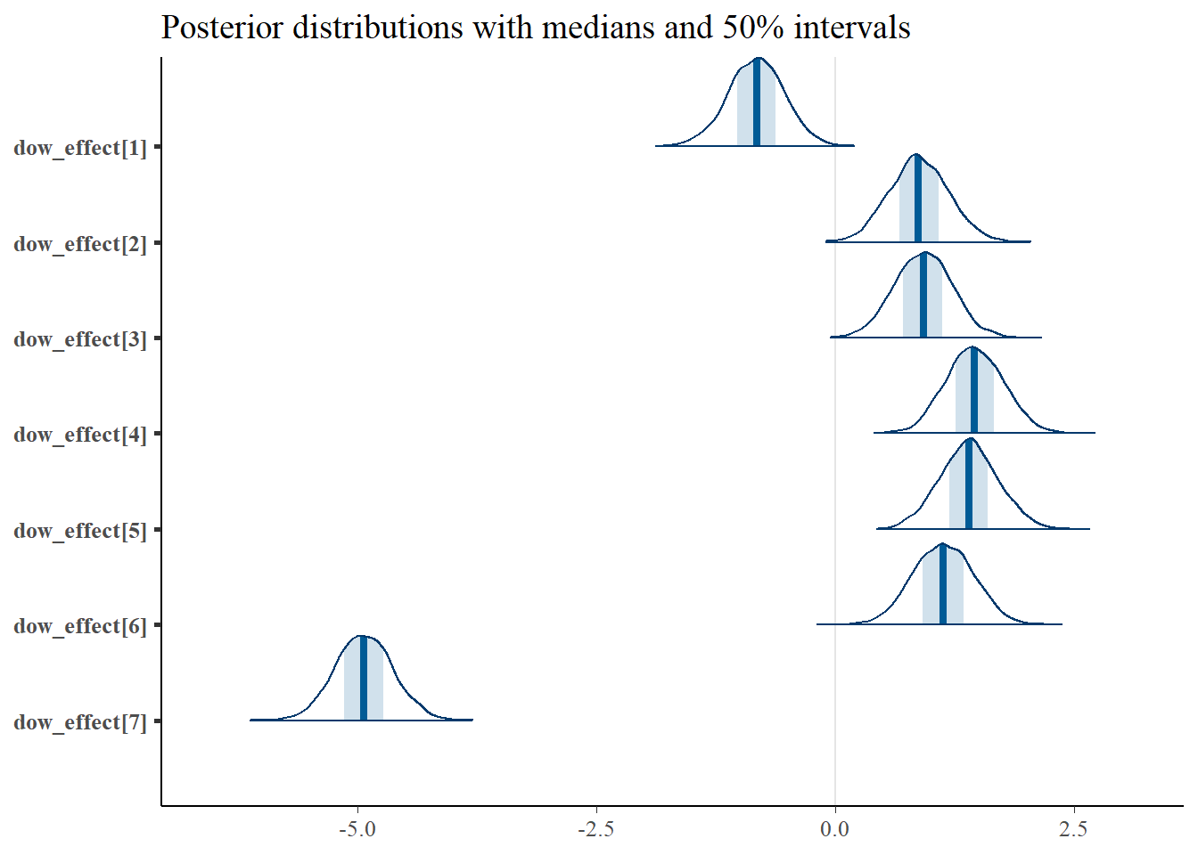
Recall that wday returns 7 on Saturdays. It turns out that Saturdays are the slowest days in terms of departing flights, followed by Sundays. Travel, at least departing from GSP, is higher during the weekdays, with the highest on Wednesdays. An airport administrator might guess this would be due to the fact that business travel occurs mostly during the week, and during the summer and holidays where vacation travel dominates (presumably), families would rather do things other than travel on Saturdays and Sundays.
Discussion
We had our first run-in with model trouble last time, and we fixed it with reparameterization. Reparameterization turns out to be a very important tool in computational Bayesian analysis (i.e. using Stan, BUGS, or even your own hand-coded MCMC routine). Here we fixed a problem with identifiability, and in this simple case that fixed a problem with the algorithm.
It’s time to step back and take stock of what’s happened so far in this series. We had a set of data that looked like it had an interesting pattern. We took the following steps with it:
- Plotted it
- Fit a simple model to it using some basic prior estimates from our knowledge
- Fit a more complex model because of a pattern we thought we recognized in the data
- Fit an even more complex model because of another pattern we thought we recognized in the data
- Saw some issues with that model, took a step back, and reparameterized to fix both some conceptual and computation issues
The last two steps might repeat many times, and while that is going on it will be helpful to revisit the objectives of the analysis. We’re going to iterate this adding complexity one more time because of one nagging feeling. We modeled the number of flights with a normal distribution because of convenience, but the number of flights is not a continuous variable. We would rather use something that can model count data.