More complex models for analyzing flight data
Introduction
In previous posts on Stan, we examined a dataset of flight departures from GSP international airport. We fit and interpreted a very simple model (simple mean plus random variation). We discussed one (very poor) way to set a prior distribution on this mean, but we hedged our bets by putting a very wide standard deviation on that prior. Then we examined the output from Stan to start discussing diagnostics. Because our model was simple, the diagnostics looked pretty good, but going forward we need to be on the lookout for issues.
In this post, we will extend the simple mean model to look at factors that might influence the number of flights. We start with the weekday - this is reasonable because the nature of travel is different on the weekend and during the week. We then add in the quarter (e.g. Jan-Mar is Q1, Apr-Jun is Q2). This turns out to be a lot like the analysis of variance (ANOVA) and other general linear models (GLM).
Setup and data
library(tidyverse)
library(lubridate)
library(rstan)
library(bayesplot)
load("airline_data.RData")
airline_data %>%
  mutate(date=ymd(YEAR*10000+MONTH*100+DAY_OF_MONTH),
         wnum = floor((date - ymd(YEAR*10000+0101))/7)) ->
  airline_data

airline_data %>%
  filter(ORIGIN_AIRPORT_ID==11996) %>%
  count(date) ->
  counts_depart
options(mc.cores = parallel::detectCores())
rstan_options(auto_write = TRUE)Analysis
Let’s go back to the raw data for a minute.
counts_depart %>%
  ggplot(aes(date,n)) +
  geom_line() +
  scale_x_date(date_breaks = "1 month", date_labels = "%b %y") +
  ylab("Number of departing flights") +
  xlab("")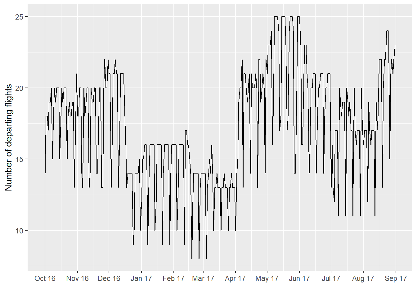
The flight count data clearly don’t “wiggle around” a constant number the whole year, but rather seem to have a complicated structure. Here’s where domain knowledge can come in handy. There are two patterns: a “high-frequency” (here, weekly) and a “low-frequency” one (here, yearly). We start with the model we had before and keep adding to it.
Adding a new mean for each quarter
Let’s review the Stan code from before:
data {
  int ndates;
  vector[ndates] flights;
}

parameters {
  real mu;
  real<lower=0> sigma;
}

model {
  flights ~ normal(mu,sigma);
  mu ~ normal(32,10);
  sigma ~ uniform(0,20);
}
The model statement, which connects our parameters to our number of flights, will clearly need to be extended. We start with the flights ~ normal(mu,sigma) statement. We are now saying that the number of flights is affected by more things, like day of week and quarter. So let’s keep it simple for now and only add quarter; say that flights ~ normal(qtr_effect,sigma). Note we eliminate mu altogether. I had actually kept it in a previous iteration, but got something that didn’t make a lot of sense. Why do you think that might be?
Now there are 4 quarters, so qtr_effect really needs to be a vector with 4 entries. So let’s try again, on the whole Stan code:
data {
  int ndates;
  vector[ndates] flights;
}

parameters {
  real<lower=0> sigma;
  vector[4] qtr_effect;
}

model {
  flights ~ normal(qtr_effect[qtr],sigma);
  sigma ~ uniform(0,20);
}
We’re almost there. We defined a vector of length 4 with our quarter effect in our parameters block, and we implemented an index for qtr_effect in the model block. We need to put a prior on our quarter effects, which we do with a for statement. For ease, we will assume the same prior on each, a normal with mean 0 and sigma of 10. The last thing we need to add is this qtr bit we added, which now has to map the day corresponding to the number of flights to an integer between 1 and 4 (so it can index qtr_effect). As we pass in number of flights as data, so must we pass in this mapping as data. So our final Stan code for number of flights accounting for quarter looks as follows:
data {
  int ndates;
  vector[ndates] flights;
  int qtr[ndates];
}

parameters {
  real<lower=0> sigma;
  vector[4] qtr_effect;
}

model {
  flights ~ normal(qtr_effect[qtr],sigma);
  sigma ~ uniform(0,20);
  for (i in 1:4)
    qtr_effect[i] ~ normal(32,10);
}
Why we represent continuous vectors as vector[length] varname and integer vectors as integer varname[length] I don’t quite get yet. But we’re done with the Stan code. I opened a text file and saved the above as flights_qtr.stan, to be called below.
Now we can proceed as the first post in this series, except now we need to define this qtr vector as the number of the quarter (from 1 to 4) that corresponds to each date and pass it to Stan. The lubridate package can make quick work of this. Remember to update data_to_pass and the file name of the Stan file.
ndates <- nrow(counts_depart)
flights <- counts_depart$n
qtr <- quarter(counts_depart$date)

data_to_pass <- c("ndates","flights","qtr")
qtr_model_fit <- stan("flights_qtr.stan",data=data_to_pass)
save(qtr_model_fit,file="qtr_model_fit.RData")
Analysis
As before, we examine the printout from qtr_model_fit:
qtr_model_fit## Inference for Stan model: flights_qtr.
## 4 chains, each with iter=2000; warmup=1000; thin=1;
## post-warmup draws per chain=1000, total post-warmup draws=4000.
##
## mean se_mean sd 2.5% 25% 50% 75% 97.5%
## sigma 3.13 0.00 0.12 2.90 3.04 3.12 3.21 3.37
## qtr_effect[1] 13.86 0.00 0.33 13.21 13.64 13.86 14.08 14.48
## qtr_effect[2] 20.20 0.00 0.32 19.59 19.99 20.20 20.42 20.84
## qtr_effect[3] 17.71 0.01 0.40 16.94 17.44 17.71 17.98 18.50
## qtr_effect[4] 17.52 0.00 0.33 16.88 17.30 17.52 17.73 18.16
## lp__ -553.91 0.03 1.55 -557.67 -554.72 -553.60 -552.79 -551.84
## n_eff Rhat
## sigma 4972 1
## qtr_effect[1] 4671 1
## qtr_effect[2] 4959 1
## qtr_effect[3] 4811 1
## qtr_effect[4] 5140 1
## lp__ 2223 1
##
## Samples were drawn using NUTS(diag_e) at Tue Jan 08 16:28:06 2019.
## For each parameter, n_eff is a crude measure of effective sample size,
## and Rhat is the potential scale reduction factor on split chains (at
## convergence, Rhat=1).As we did last time, we look at traceplots before saying too much more. (Note also that Rhat=1 for each of the parameters above, so that looks pretty good.) Because we have a vector, and it would be a pain in the hindside to type out all of the qtr_effect[1] ... qtr_effect[4] parameters, we use the regex_pars option of mcmc_trace to examine the trace plots.
p <- mcmc_trace(as.array(qtr_model_fit),pars="sigma",regex_pars = "qtr_effect",
                facet_args = list(nrow = 5, labeller = label_parsed))
p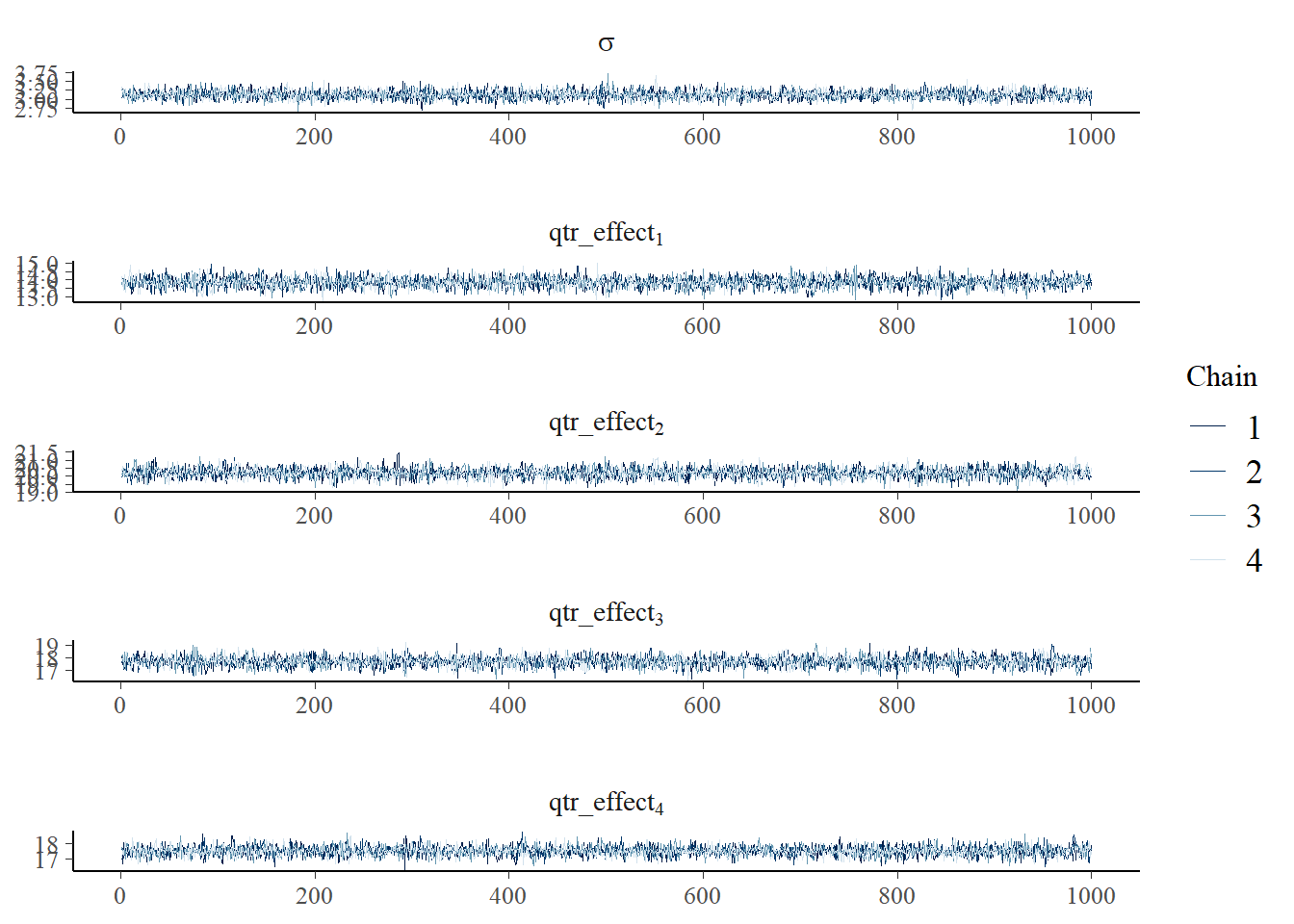
Things look pretty good, so we can proceed. We look at density plots as well, with the same bit of trickery with regex_pars as above:
p <- mcmc_areas(as.matrix(qtr_model_fit),pars="sigma",regex_pars = "qtr_effect",prob = 0.5) +
  ggtitle("Posterior distributions with medians and 50% intervals")
p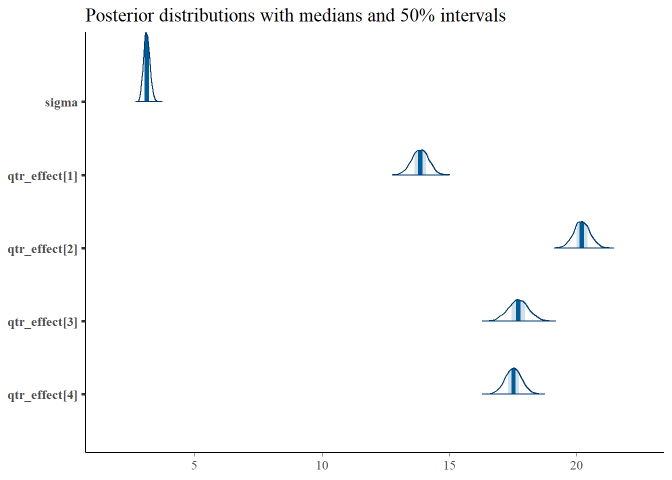
Now we can plainly see that in Quarter 2, the number of flights is much higher, averaging around 20 departures per day (perhaps due to all the summer vacations), with a pullback in Quarters 3 and 4, and with a lot less in Quarter 1.
Adding a second explanatory variable
Using the same reasoning as above, we can add a weekday effect. It would be instructive to work your way through the reasoning, so I present the final Stan code here. (Hint: I started with the flights ~ statement in the model block to start the addition.)
data {
  int ndates;
  vector[ndates] flights;
  int qtr[ndates];
  int dow[ndates];
}

parameters {
  real<lower=0> sigma;
  vector[4] qtr_effect;
  vector[7] dow_effect;
}

model {
  flights ~ normal(qtr_effect[qtr] + dow_effect[dow],sigma);
  sigma ~ uniform(0,20);
  for (i in 1:4)
    qtr_effect[i] ~ normal(32,10);
  for (i in 1:7)
    dow_effect[i] ~ normal(0,10);
}
And here is the updated R code to call the new model:
ndates <- nrow(counts_depart)
flights <- counts_depart$n
qtr <- quarter(counts_depart$date)
dow <- wday(counts_depart$date)

data_to_pass <- c("ndates","flights","qtr","dow")
qtr_dow_model_fit <- stan("flights_qtr_dow.stan",data=data_to_pass)
save(qtr_dow_model_fit,file="qtr_dow_model_fit.RData")
qtr_dow_model_fit
## Inference for Stan model: flights_qtr_dow.
## 4 chains, each with iter=2000; warmup=1000; thin=1;
## post-warmup draws per chain=1000, total post-warmup draws=4000.
##
## mean se_mean sd 2.5% 25% 50% 75% 97.5%
## sigma 2.29 0.00 0.10 2.11 2.22 2.28 2.35 2.49
## qtr_effect[1] 19.08 0.15 2.91 13.24 17.04 19.20 20.95 24.79
## qtr_effect[2] 25.47 0.15 2.92 19.61 23.47 25.61 27.35 31.22
## qtr_effect[3] 23.01 0.15 2.92 17.18 21.03 23.12 24.90 28.72
## qtr_effect[4] 22.84 0.15 2.90 16.97 20.82 22.98 24.69 28.53
## dow_effect[1] -6.08 0.15 2.92 -11.81 -7.98 -6.17 -4.06 -0.26
## dow_effect[2] -4.37 0.15 2.92 -10.08 -6.28 -4.47 -2.38 1.53
## dow_effect[3] -4.34 0.15 2.93 -10.07 -6.21 -4.47 -2.31 1.59
## dow_effect[4] -3.79 0.15 2.93 -9.53 -5.67 -3.92 -1.74 2.12
## dow_effect[5] -3.86 0.15 2.92 -9.59 -5.74 -3.97 -1.85 2.07
## dow_effect[6] -4.13 0.15 2.92 -9.78 -6.03 -4.22 -2.08 1.76
## dow_effect[7] -10.17 0.15 2.92 -15.88 -12.06 -10.28 -8.17 -4.30
## lp__ -446.51 0.09 2.56 -452.63 -447.95 -446.14 -444.64 -442.62
## n_eff Rhat
## sigma 889 1
## qtr_effect[1] 369 1
## qtr_effect[2] 370 1
## qtr_effect[3] 366 1
## qtr_effect[4] 371 1
## dow_effect[1] 372 1
## dow_effect[2] 376 1
## dow_effect[3] 368 1
## dow_effect[4] 372 1
## dow_effect[5] 373 1
## dow_effect[6] 370 1
## dow_effect[7] 374 1
## lp__ 847 1
##
## Samples were drawn using NUTS(diag_e) at Tue Jan 08 16:28:12 2019.
## For each parameter, n_eff is a crude measure of effective sample size,
## and Rhat is the potential scale reduction factor on split chains (at
## convergence, Rhat=1).You’ll notice the model is starting to have a harder time, with Rhat = 1.01 for all the effects. This model is perfectly ok, for the most part (look at the mcmc_trace!), but we’ll talk next time about a subtle issue with it (and one I easily swept under the rug earlier when adding a quarter effect). Hint: it had to do with a previous iteration of this post I talked about above.
Discussion
After having introduced the Greenville flight data, a simple model for analysis, and how to analyze output, we discussed how to exploit some of the structure in the data, specifically the fact that airlines tend to run flights by seasons and day of week. We saw how this manifested in the Stan code, working from the model block back to the data block. But there are storm clouds on the horizon, as we started getting some curious results and some more difficulty with convergence.