Federal R&D

The first dataset shows Federal R&D, and looks as follows:

head(fed_rd)

## # A tibble: 6 x 7
##   department  year  rd_budget total_outlays discretionary_ou~     gdp party
##   <chr>      <dbl>      <dbl>         <dbl>             <dbl>   <dbl> <chr>
## 1 DOD         1976    3.57e10  371800000000      175600000000 1.79e12 Repu~
## 2 NASA        1976    1.25e10  371800000000      175600000000 1.79e12 Repu~
## 3 DOE         1976    1.09e10  371800000000      175600000000 1.79e12 Repu~
## 4 HHS         1976    9.23e 9  371800000000      175600000000 1.79e12 Repu~
## 5 NIH         1976    8.02e 9  371800000000      175600000000 1.79e12 Repu~
## 6 NSF         1976    2.37e 9  371800000000      175600000000 1.79e12 Repu~

This already suggests a visualization, so let’s try one. The default y-axis label is in dollars, so I use the scales::dollar_format function to scale it to billions of dollars, and adjust the label accordingly.

ggplot(fed_rd, aes(year, rd_budget, group = department, color = department)) +
  geom_line() +
  geom_rect(aes(xmin = from, xmax = to, ymin = -Inf, ymax = Inf, fill = party), 
            inherit.aes = FALSE, data = party, alpha = 0.2) +
  xlab("Year") +
  ylab("Federal R&D Budget (billions)") +
  scale_color_viridis_d() +
  scale_fill_brewer() +
  scale_y_continuous(labels = scales::dollar_format(scale = 1e-9))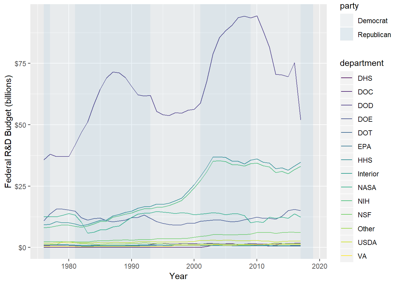

It would be interesting to get these budgets as a percentage of discretionary or total outlays. We’ll start with discretionary. I use the scales::percent_format to label the y-xaxis. The automatic guess from scales::percent gives one decimal place, which I thought was silly for this graph, so I put in the extra effort to cut it out.

fed_rd %>% 
  mutate(rd_perc_disc = rd_budget / discretionary_outlays) %>% 
  ggplot(aes(year, rd_perc_disc, group = department, color = department)) +
  geom_line() +
  geom_rect(aes(xmin = from, xmax = to, ymin = -Inf, ymax = Inf, fill = party), 
            inherit.aes = FALSE, data = party, alpha = 0.2) +
  xlab("Year") +
  ylab("Federal R&D proportion of discretionary spending") +
  scale_colour_viridis_d() +
  scale_fill_brewer() +
  scale_y_continuous(labels = scales::percent_format(accuracy = 1))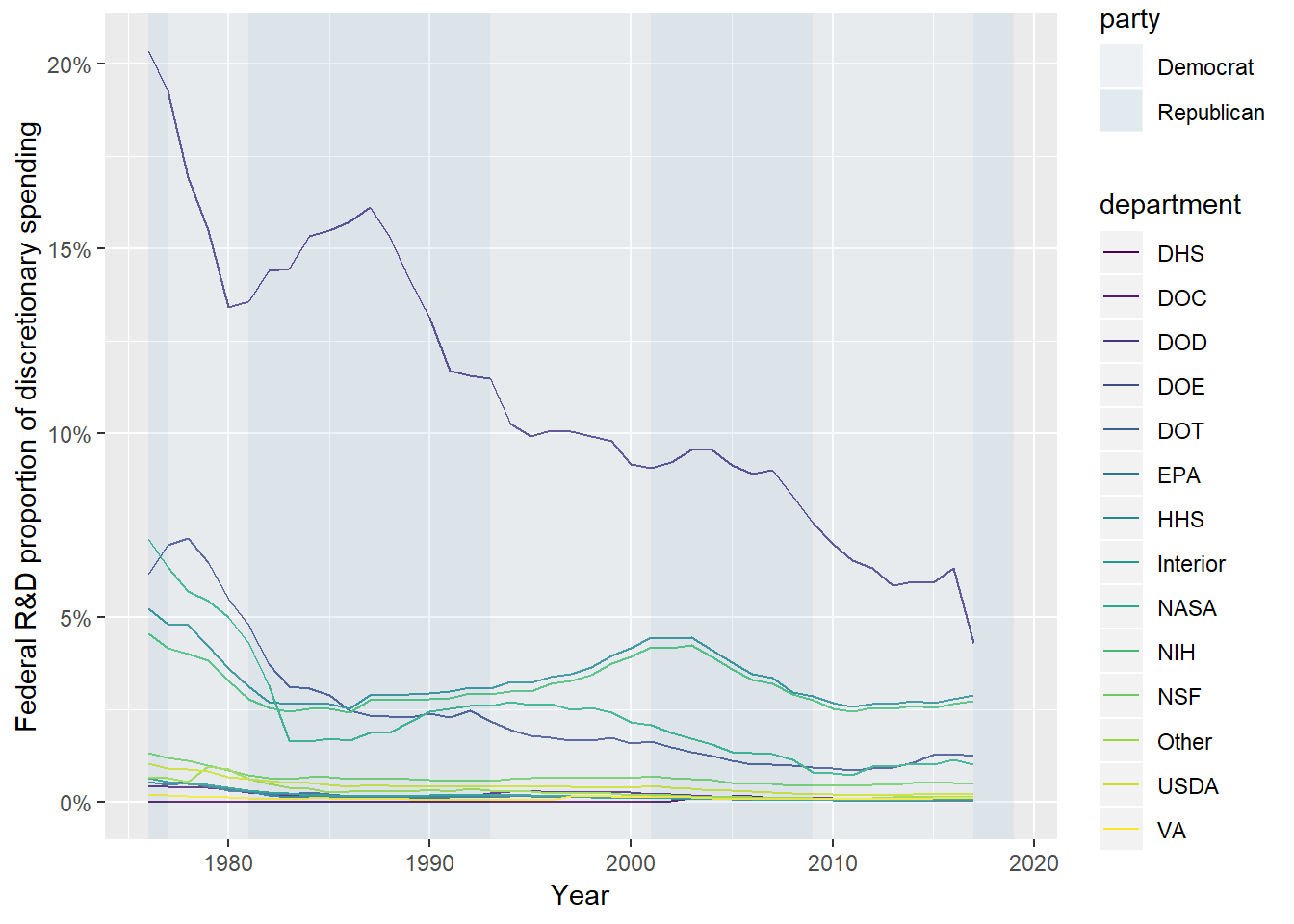

The same for percentage of total, leaving the extra decimal place in this time because it is informative:

fed_rd %>% 
  mutate(rd_perc_tot = rd_budget / total_outlays) %>% 
  ggplot(aes(year, rd_perc_tot, group = department, color = department)) +
  geom_line() +
  geom_rect(aes(xmin = from, xmax = to, ymin = -Inf, ymax = Inf, fill = party), 
            inherit.aes = FALSE, data = party, alpha = 0.2) +
  xlab("Year") +
  ylab("Federal R&D proportion of total spending") +
  scale_colour_viridis_d() +
  scale_fill_brewer() +
  scale_y_continuous(labels = scales::percent)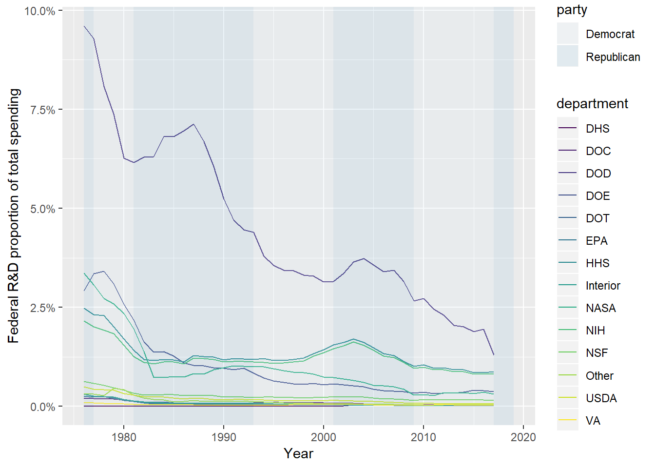 

Ok, so this brief exploration showed that defense spending has dominated other spending, at least as a portion of the federal budget. One thing I did check on at the AAAS site is that this spending is adjusted for inflation. (Probably should have checked that before embarking on this!)

I think it is worth trying to remake the above graph but switching the legend order based on the average spending over time. Here we go:

fed_rd %>% 
  mutate(rd_perc_tot = rd_budget / total_outlays,
         department = fct_reorder(department, rd_perc_tot, .fun = mean)) %>% 
  ggplot(aes(year, rd_perc_tot, group = department, color = department)) +
  geom_line() +
  geom_rect(aes(xmin = from, xmax = to, ymin = -Inf, ymax = Inf, fill = party), 
            inherit.aes = FALSE, data = party, alpha = 0.2) +
  xlab("Year") +
  ylab("Federal R&D proportion of total spending") +
  scale_colour_viridis_d(option = "B", direction = -1) +
  scale_fill_brewer() +
  scale_y_continuous(labels = scales::percent)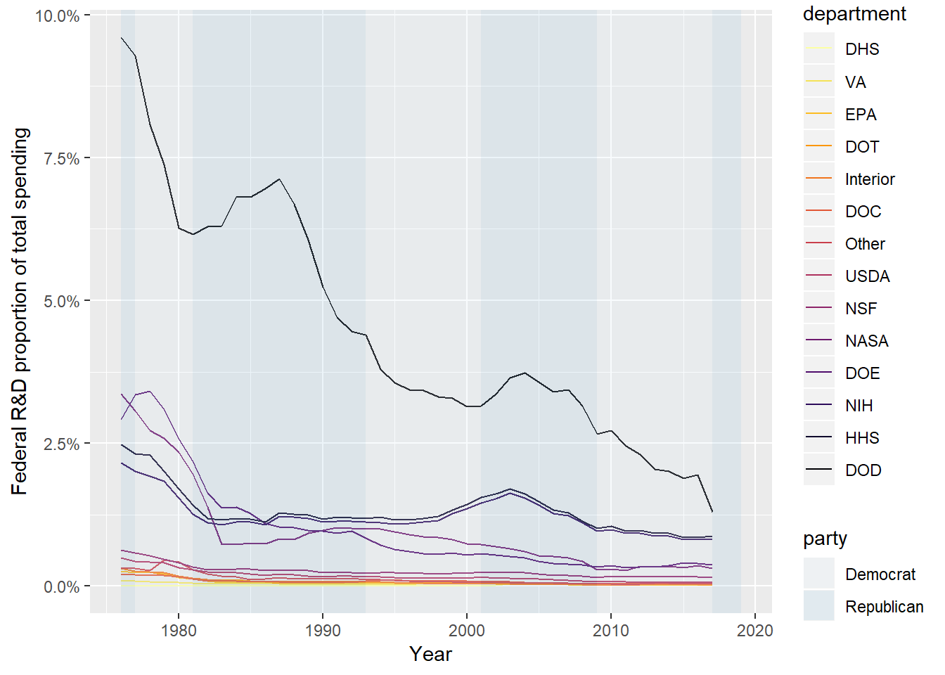 

I think this graph is more informative than the above graph ordered alphabetically by department. I also switched up the color scheme a bit. To me this subtle change made the graph far more informative, with the color legend giving the order of the priority (more or less) of R&D vs the discretionary spending from least to most. This simple change using the fct_reorder function from the forcats package (loaded as part of tidyverse) is very powerful. (I could have also done this in the ggplot aesthetic.)

One more quick addition to see if it adds anything:

fed_rd %>% 
  mutate(rd_perc_tot = rd_budget / total_outlays,
         department = fct_reorder(department, rd_perc_tot, .fun = mean)) %>% 
  ggplot(aes(year, rd_perc_tot, group = department, color = department)) +
  geom_line() +
  geom_rect(aes(xmin = from, xmax = to, ymin = -Inf, ymax = Inf, fill = party), 
            inherit.aes = FALSE, data = party, alpha = 0.2) +
  geom_smooth(method = "lm", se = FALSE, size = 0.5, linetype = "dotted") +
  xlab("Year") +
  ylab("Federal R&D proportion of total spending") +
  scale_colour_viridis_d(option = "B", direction = -1) +
  scale_fill_brewer() +
  scale_y_continuous(labels = scales::percent)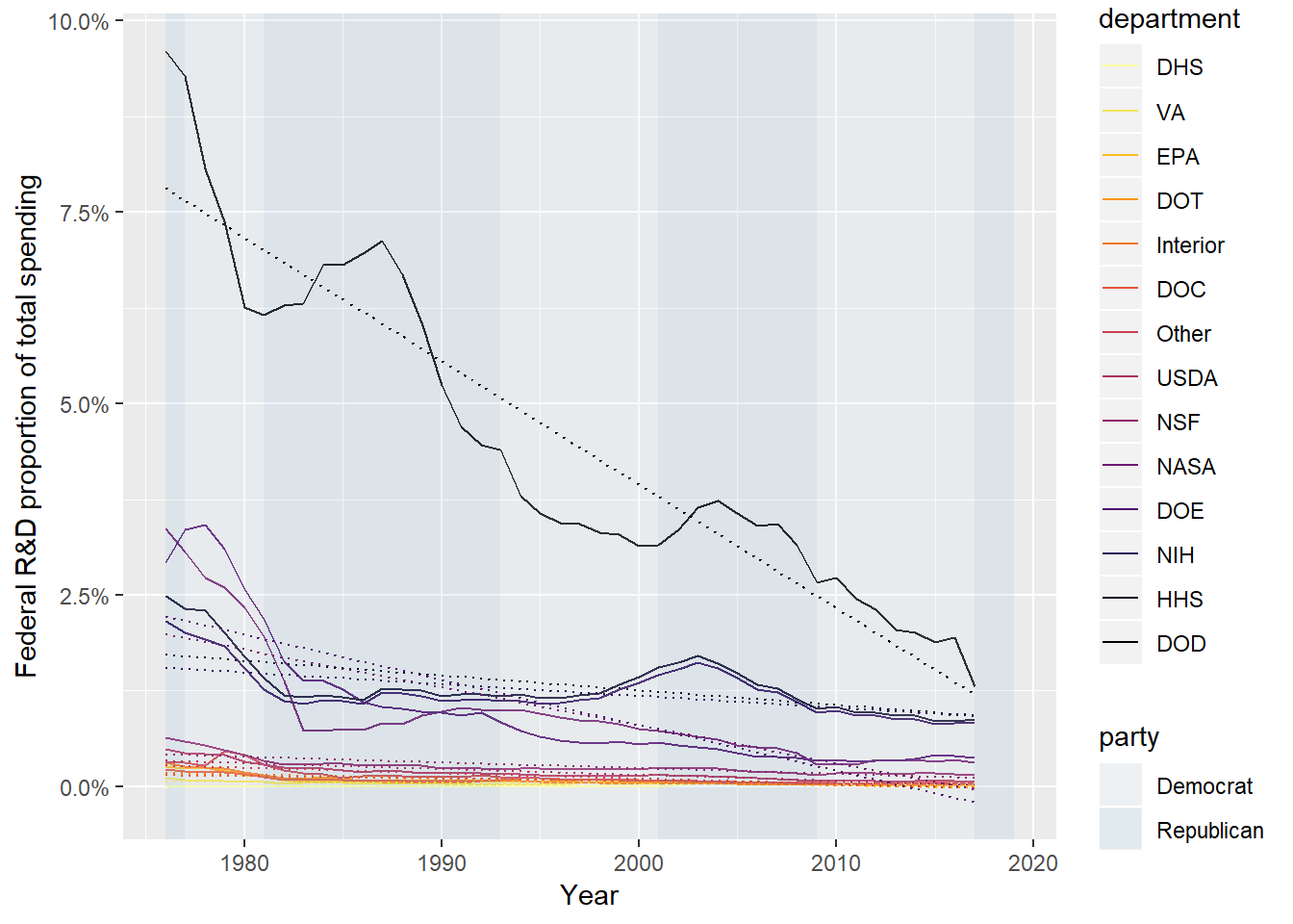 

The fitted lines give a little more information that may help group the R&D budgets even further. We have DOD, in a class by itself (obvious from the raw line plot), HHS and NIH that have a slight trend down over time, DOE and NASA that started higher but have a stronger trend down, then everything else that started low relative to everything else and as a result remain relatively flat. One final picture, putting the y-axis on log scale:

fed_rd %>% 
  mutate(rd_perc_tot = rd_budget / total_outlays,
         department = fct_reorder(department, rd_perc_tot, .fun = mean)) %>% 
  ggplot(aes(year, rd_perc_tot, group = department, color = department)) +
  geom_line() +
  geom_rect(aes(xmin = from, xmax = to, ymin = 0.0001, ymax = Inf, fill = party), 
            inherit.aes = FALSE, data = party, alpha = 0.2) +
  geom_smooth(method = "lm", se = FALSE, size = 0.5, linetype = "dotted") +
  xlab("Year") +
  ylab("Federal R&D proportion of total spending") +
  scale_colour_viridis_d(option = "B", direction = -1) +
  scale_fill_brewer() +
  scale_y_log10(labels = scales::percent) 

## Warning: Transformation introduced infinite values in continuous y-axis

## Warning: Transformation introduced infinite values in continuous y-axis

## Warning: Removed 26 rows containing non-finite values (stat_smooth).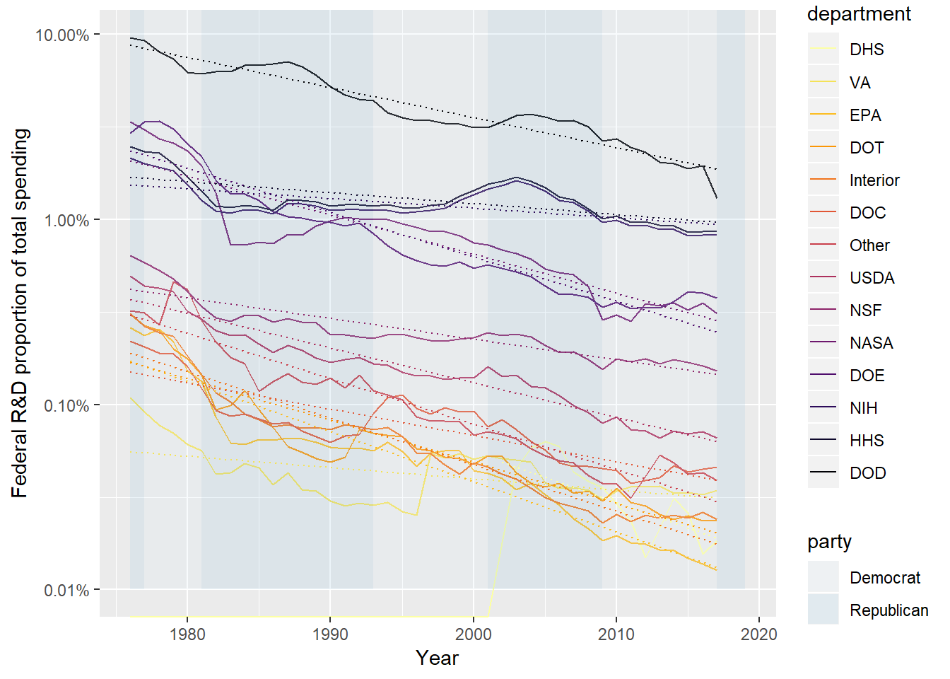

This graph was produced by switching scale_y_log10 in for scale_y_continuous. You get a whole bunch of junk complaining about how you can’t take the log of a negative values (from geom_smooth, because the linear trend extends below 0), and geom_rect if you keep the ymin = -Inf. I went ahead and changed ymin = 0.01 so we could keep the party shading. The main effect of the log scale was to explore the trends of the “everything else” in the above graphs. What was a relatively flat trend still is, but it is shown that everything in R&D is trending down relative to discretionary spending.

These three graphs all give an interesting picture. Under Republican presidents in general, defense R&D spending has increased, sometimes drastically so, for a few years and started to fall. But as a general trend, defense spending as a percentage of discretionary and total spending has declined since the 1970s, where we were still in the heat of the Cold War. (It’s important to remember we’re talking about R&D spending.)