Cancer rates in SC - introduction to the tidybayes package
Introduction and Purpose
In the last series of examples, I focused on Bayesian modeling using the Stan package. This useful package on the surface makes Bayesian analysis a lot easier, but from my point of view the real power (of this and other packages such as JAGS and BUGS) is the ability to specify a model directly from the science and a few statistical ideas. I placed less emphasis on diagnostics, evaluation, and interpretation of the model. In this series I go further into these topics.
The data
I want to use a second example for this series, and I have chosen new cancer cases by county in South Carolina. This data is available for download from the website for the South Carolina Environmental Public Health Tracking program. You can choose new cases, age-adjusted new cases, new cases over 5 years, and other criteria. I chose just the new cases. It will bring up a chloropleth map when you make your selection, but you can pull up a table and download it. Be careful – though they say it’s for Excel, it’s really an HTML table with some extra parts.
First, the setup:
library(tidyverse)
library(viridis)
library(rvest)
library(xml2)
library(stringr)
library(rstanarm)
library(tidybayes)

options(mc.cores = 4)
`%nin%` <- function (x, table) match(x, table, nomatch = 0L) == 0L
I load the tidyverse for data manipulation, viridis for some visualization, rvest and xml2 to read data off the web (or web data downloaded locally), stringr for more data cleaning, and rstanarm and tidybayes for analysis.
I also define the %nin% function which will help us filter parameters later on. You could also load the Hmisc package, which is otherwise excellent, but I wanted to go lightweight here.
New cancer cases
I’ve already downloaded the cancer data to my local drive, but it is in the original state. I load and clean that data here. Then I show a quick visualization. I won’t show the legends in these quick visualizations because they will take up too much space.
new_cancer <- xml2::read_html("data/cancer_cases_new_sc_2010-2014.xls") %>%
  html_node("table") %>%
  html_table(fill = TRUE) %>%
  slice(3:49) %>%
  `names<-`(c("county", 2001:2014)) %>%
  gather(year,new_cases,starts_with("2")) %>%
  mutate(new_cases = as.numeric(new_cases),
         year = as.numeric(year))

new_cancer %>%
  ggplot(aes(x = year, y = new_cases, group = county)) +
  geom_line()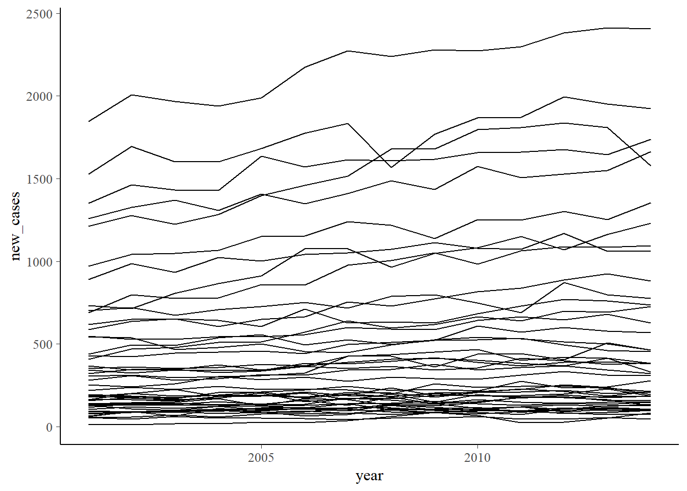
Population
If you notice in the visualization, there are some counties that have a lot of cases of cancer! If you’re an epidemiologist or have had other statistical training, your next natural question is “but what is the population in those counties”? After all, we want to look at new cancer rates, not raw cases. So we download the population. This data is based on Census estimates, and contains both intercensus estimates (2001 – 2010) and postcensus estimates (2011 – 2014). We ignore the differences of estimates between censuses and those after the last census (interpolation vs. extrapolation), and treat them all as estimates on equal footing, but they are in different tables and have to be put together. These data can be found on the SC state government website. We also give a quick visualization.
# get population information, downloaded from
# http://abstract.sc.gov/chapter14/pop5.html
sc_pop_county_est1 <- xml2::read_html("http://abstract.sc.gov/chapter14/pop6.html") %>%
  html_node("table") %>%
  html_table() %>%
  `names<-`(c("county", 2000:2009)) %>%
  filter(!(county %in% c("South Carolina", "South  Carolina")))

sc_pop_county_est2 <- xml2::read_html("http://abstract.sc.gov/chapter14/pop7.html") %>%
  html_node("table") %>%
  html_table() %>%
  select(1:6) %>%
  `names<-`(c("county", 2010:2014)) %>%
  filter(!(county %in% c("South Carolina", "South  Carolina")))

sc_pop_county_est <- sc_pop_county_est1 %>%
  full_join(sc_pop_county_est2) %>%
  gather(year, est_pop, -1) %>%
  mutate(year = as.numeric(year),
         est_pop = as.numeric(str_remove(est_pop,",")))
## Joining, by = "county"sc_pop_county_est %>%
ggplot(aes(x = year, y = est_pop, group = county)) +
geom_line() + scale_y_log10()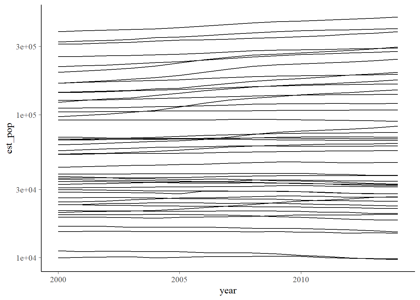
Cancer rates
Now we combine the two datasets from above.
new_cancer %>%
  full_join(sc_pop_county_est %>% filter(year > 2000)) %>%
  mutate(new_case_rate = new_cases / est_pop) %>%
  filter(county != "Unknown") %>%
  mutate(year_mod = year - 2000,
         log_pop = log(est_pop)) ->
  new_cancer_rate
## Joining, by = c("county", "year")If you notice, I added two new variables to the dataset. I did that mostly for efficiency later on, but this was something I added rather late into the analysis process. I’ll explain year_mod and log_pop when I get to the analysis. Don’t worry about them for now.
Preliminary analysis
There are a lot of questions we can now ask of this dataset. First, a quick visualization.
new_cancer_rate %>%
  ggplot(aes(x = year, y = new_case_rate, group = county)) +
  geom_line() +
  scale_color_viridis(discrete = TRUE) +
  scale_y_log10()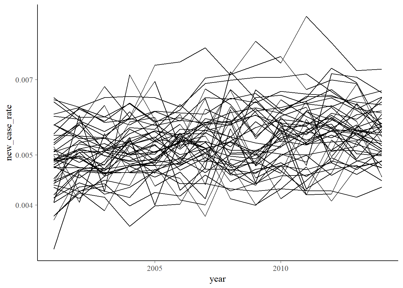
Though having little to do with Bayesian analysis, we might take a quick peek at who had the best and worst cancer rates over the years. Here’s the worst:
new_cancer_rate %>%
  group_by(year) %>%
  mutate(county_rank = rank(new_case_rate, na.last = FALSE, ties.method = "first")) %>%
  summarize(county = county[county_rank == min(county_rank, na.rm = TRUE)],
            new_case_rate = max(new_case_rate, na.rm=TRUE))
## # A tibble: 14 x 3
## year county new_case_rate
## <dbl> <chr> <dbl>
## 1 2001 Saluda 0.00646
## 2 2002 Allendale 0.00619
## 3 2003 Edgefield 0.00679
## 4 2004 Jasper 0.00715
## 5 2005 Jasper 0.00746
## 6 2006 Jasper 0.00757
## 7 2007 Allendale 0.00807
## 8 2008 Dillon 0.00725
## 9 2009 Dillon 0.00830
## 10 2010 Edgefield 0.00776
## 11 2011 Hampton 0.00928
## 12 2012 Jasper 0.00826
## 13 2013 Richland 0.00729
## 14 2014 Richland 0.00734And here’s the best:
new_cancer_rate %>%
  group_by(year) %>%
  mutate(county_rank = rank(new_case_rate, na.last = FALSE, ties.method = "first")) %>%
  summarize(county = county[county_rank == max(county_rank, na.rm = TRUE)],
            new_case_rate = min(new_case_rate, na.rm=TRUE))
## # A tibble: 14 x 3
## year county new_case_rate
## <dbl> <chr> <dbl>
## 1 2001 Georgetown 0.00328
## 2 2002 Oconee 0.00405
## 3 2003 McCormick 0.00390
## 4 2004 Calhoun 0.00364
## 5 2005 McCormick 0.00398
## 6 2006 McCormick 0.00402
## 7 2007 McCormick 0.00380
## 8 2008 Calhoun 0.00412
## 9 2009 McCormick 0.00399
## 10 2010 Georgetown 0.00411
## 11 2011 McCormick 0.00418
## 12 2012 McCormick 0.00407
## 13 2013 McCormick 0.00414
## 14 2014 McCormick 0.00434You’ll see the same names popping up over and over in these superlatives analysis, and it might be an interesting question as to why these counties have such good or bad rates. Explanations might range from some counties may be retirement destinations for people less likely to get cancer to something more nefarious like pollution. Or you might worry about smoking rates by county. But that’s not in our dataset.
Modeling
Now we get to the good stuff. The model here will be a Poisson regression with an offset. Why? The Poisson regression part comes from the fact that we are modeling count data. (We could have also used the more general negative binomial model that was the final one we used with the flight dataset.) The offset is something you may not have encountered before. You use it when you are looking at Poisson rates with varying levels of exposure. Here, we have counties with varying levels of population (and those levels vary over the years for each county). You would also use an offset if you are looking at the incidence of adverse events in patients on a particular treatment because patients have different amounts of times they are exposed to treatment. You might also use offsets to compare customer rates in stores that have varying amounts of time that they are open. The trick to offsets is that you have to take the logarithm of the “exposure” - in this case population. Now you see why I created log_pop in the dataset above. The reason we have to do this is because with Poisson regression, we use the log link function.
While I’m on theory, let me explain the year_mod variable. I plan to look at the change in new cancer case rates over time. Our dataset begins in 2001, but if I use a raw year in the model, the sampling algorithm may get confused and/or the scaling of parameters based on year might look strange. It’s better to represent year in, say, number of years after 2000 (as I did).
Ok, with that long-winded explanation out of the way, let’s get to the modeling. I mentioned last time you can use the rstanarm package to do the modeling. This is useful because you don’t have to worry as much about the details of running Stan and can use a familiar syntax. (Side note: you do have to worry about some details. At one point I forgot to take the log of the population to use as an offset. Stan refused to run the model. It took a bit of time before I realized my mistake.) For priors we will use normal distributions that cover reasonable values for our parameters. If you are worried about strange values, you could use a Student \(t\) or even go wild and crazy with a Cauchy. Now the prior affects our county and year parameters, but they may not be on the same scale as the intercept. Thus, rstanarm offers the prior_intercept so you can put a reasonable prior on all your parameters.
bayes_pois_fit <- new_cancer_rate %>%
  stan_glm(new_cases ~ year_mod + county + offset(log_pop),
           family = poisson(link = "log"),
           data = .,
           prior = normal(0,1),
           prior_intercept = normal(0,5))

bayes_pois_fit
## stan_glm
## family: poisson [log]
## formula: new_cases ~ year_mod + county + offset(log_pop)
## observations: 644
## predictors: 47
## ------
## Median MAD_SD
## (Intercept) -5.2 0.0
## year_mod 0.0 0.0
## countyAiken -0.2 0.0
## countyAllendale -0.2 0.0
## countyAnderson 0.0 0.0
## countyBamberg 0.0 0.0
## countyBarnwell -0.2 0.0
## countyBeaufort 0.1 0.0
## countyBerkeley -0.2 0.0
## countyCalhoun 0.0 0.0
## countyCharleston -0.1 0.0
## countyCherokee -0.1 0.0
## countyChester 0.0 0.0
## countyChesterfield -0.1 0.0
## countyClarendon 0.0 0.0
## countyColleton 0.1 0.0
## countyDarlington -0.1 0.0
## countyDillon -0.2 0.0
## countyDorchester -0.2 0.0
## countyEdgefield -0.2 0.0
## countyFairfield 0.0 0.0
## countyFlorence -0.1 0.0
## countyGeorgetown 0.2 0.0
## countyGreenville -0.1 0.0
## countyGreenwood 0.0 0.0
## countyHampton -0.1 0.0
## countyHorry 0.1 0.0
## countyJasper -0.3 0.0
## countyKershaw 0.0 0.0
## countyLancaster -0.1 0.0
## countyLaurens 0.0 0.0
## countyLee -0.1 0.0
## countyLexington -0.2 0.0
## countyMarion -0.1 0.0
## countyMarlboro -0.1 0.0
## countyMcCormick 0.3 0.0
## countyNewberry 0.0 0.0
## countyOconee 0.2 0.0
## countyOrangeburg 0.0 0.0
## countyPickens -0.1 0.0
## countyRichland -0.3 0.0
## countySaluda -0.1 0.0
## countySpartanburg -0.1 0.0
## countySumter -0.1 0.0
## countyUnion 0.1 0.0
## countyWilliamsburg 0.0 0.0
## countyYork -0.2 0.0
##
## Sample avg. posterior predictive distribution of y:
## Median MAD_SD
## mean_PPD 502.1 1.3
##
## ------
## * For help interpreting the printed output see ?print.stanreg
## * For info on the priors used see ?prior_summary.stanregVisualization of the posterior distributions
This post is getting long, and it is getting late, but I did want to at least touch on tidybayes. While for a lot of the time the Stan community used the bayesplot package (which is very nice in some ways), tidybayes makes working with Stan fit objects feel more like working with dplyr and ggplot2.
The first plot is an easy one - just the posterior distribution of the year_mod coefficient, which will answer the question of whether new cancer incidence rates as a whole are going up over time. We’ll compare this distribution to 0.
bayes_pois_fit %>%
  tidy_draws() %>%
  gather(variable, draw, 4:ncol(.)) %>%
  filter(variable %in% c( "year_mod")) %>%
  ggplot(aes(x = draw, y = fct_reorder(variable, draw, .desc = TRUE))) +
  geom_halfeyeh(fun.data = median_hdi) +
  scale_y_discrete(labels = "") +
  ylab("") + xlab("log(relative new cancer case rate per year increase)")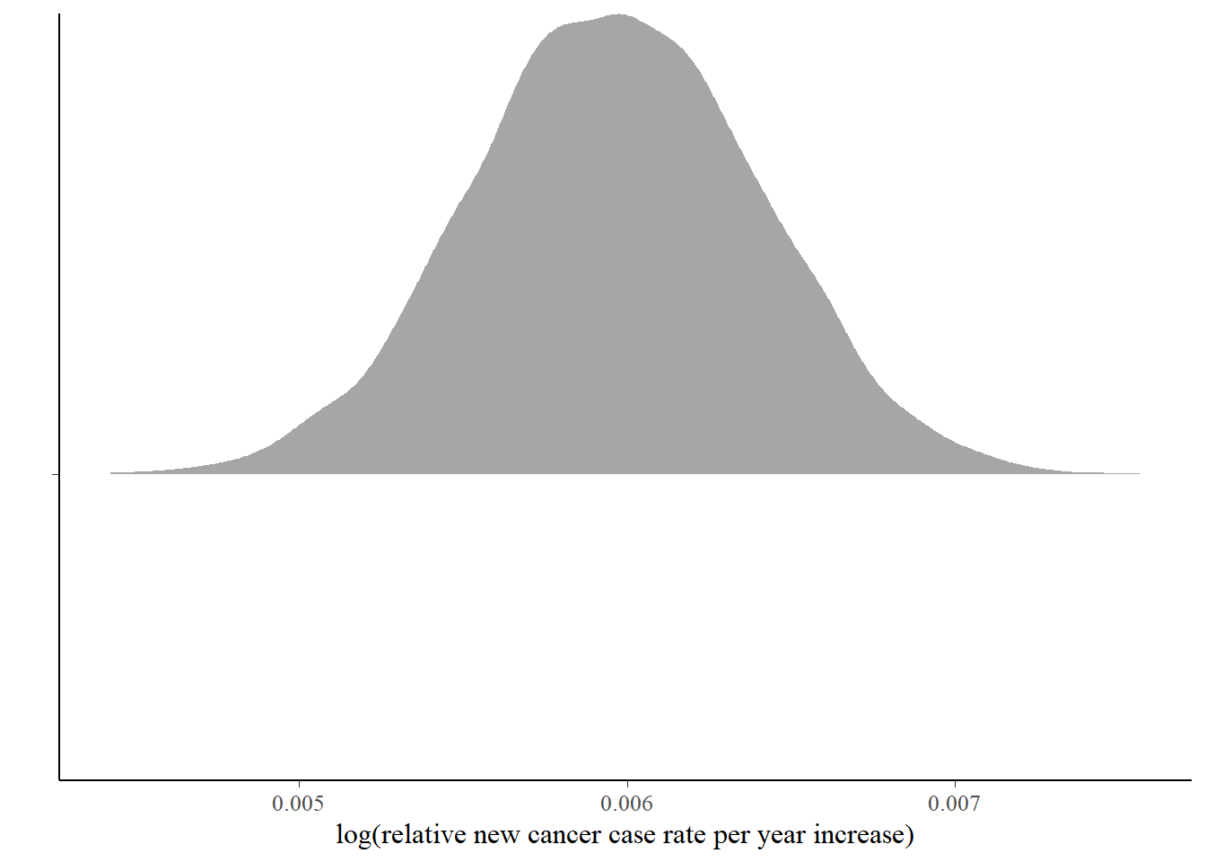
The first things to notice is that we started with the Stan fit object, and used tidy_draws to pull out the posterior samples. We’re left with a tbl_df, so this fits in with the tidy tools philosophy. We can then use tidyr and dplyr to get our data the way we want it. I should point out here that a lot of times, parameters will come out of Stan looking like parameter[a,b] or something like that. tidybayes has functions to handle those situation easily. Here we only had that one factor with 46 levels (counties), so it was just easier to use tidy_draws directly and then gather and filter in this particular case. Because you’re using tidy tools, the choice is up to you.
tidybayes also adds the geom_halfeyeh and other, similar geoms that you might want to use when you are visualizing posterior distribution draws. It also provides complementary statistics functions like median_hdi.
If you want to switch the visualization to a pointrange (density plots just aren’t your thing), you can do that easily using stat_pointinterval (or stat_pointintervalh):
bayes_pois_fit %>%
  tidy_draws() %>%
  gather(variable, draw, 4:ncol(.)) %>%
  filter(variable %in% c( "year_mod")) %>%
  ggplot(aes(x = draw, y = variable)) +
  stat_pointintervalh(.width = c(0.8, 0.95)) +
  scale_y_discrete(labels = "") +
  ylab("") + xlab("log(relative new cancer case rate per year increase)")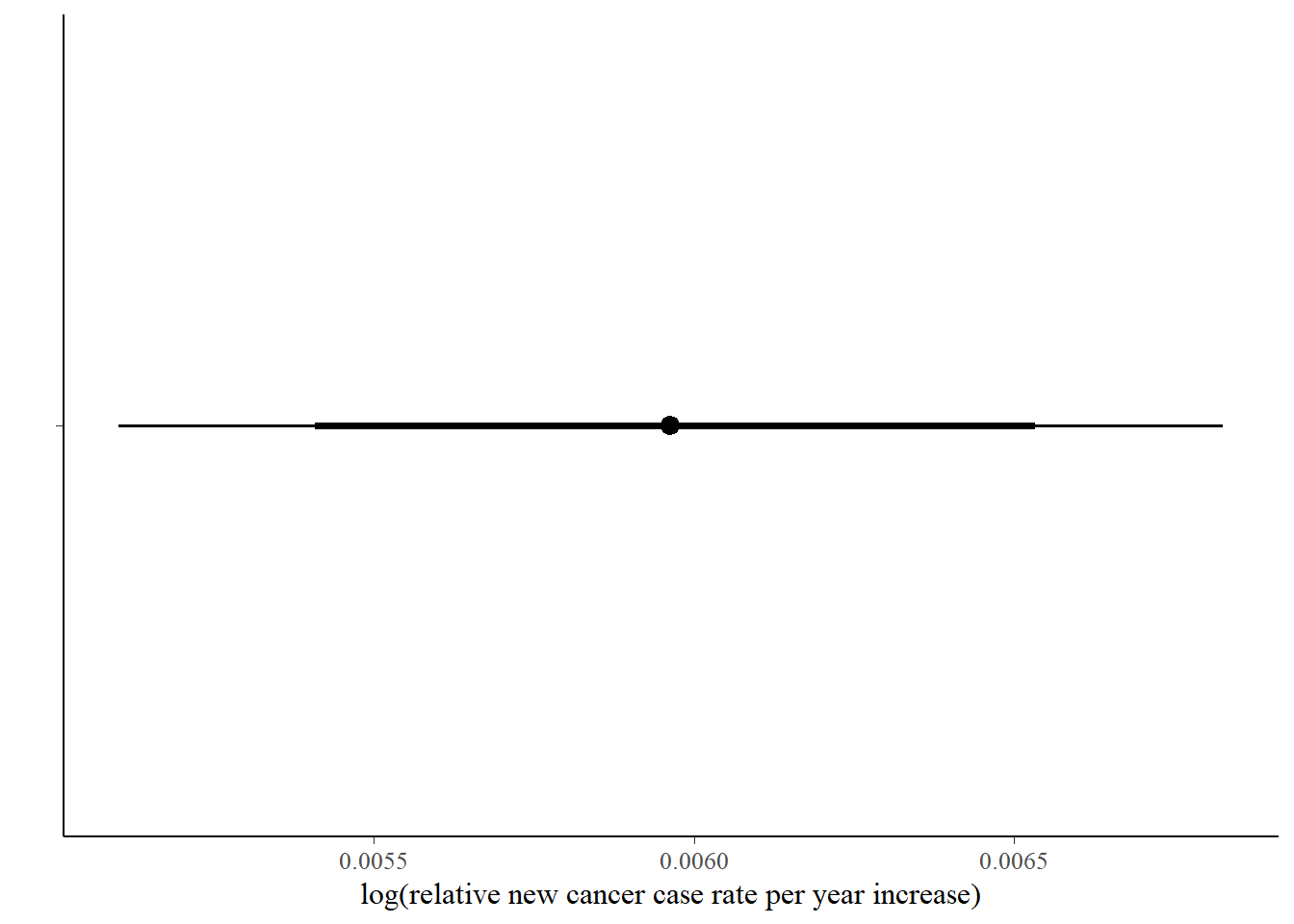
There are a couple of things I like about this approach over the bayesplot approach. Here I can piece together the graph I want in a natural ggplot2-like way. With bayesplot, you get the whole package in one command, though you can alter or add ggplot2 layers normally. But this just feels more natural in my analysis flow.
Regarding interpretation, the answer is yes, from this data, there is a very high probability that new cancer rates are going up over time, albeit slowly. (Keep in mind this is on a log scale, so the coefficient 0.006 means multiply the current new cancer rate in SC by exp(0.006) = 1.006 to get next year’s overall estimate.)
Now we get a little more fancy and look at rates by county:
bayes_pois_fit %>%
  tidy_draws() %>%
  gather(variable, draw, 4:ncol(.)) %>%
  filter(variable %nin% c("year_mod", "(Intercept)")) %>%
  ggplot(aes(x = draw, y = fct_reorder(variable, draw, .desc = TRUE))) +
  geom_halfeyeh(fun.data = median_hdi) +
  scale_y_discrete(labels = function(.x) str_remove(.x,"county")) +
ylab("County") + xlab("log(relative new cancer case rate)") 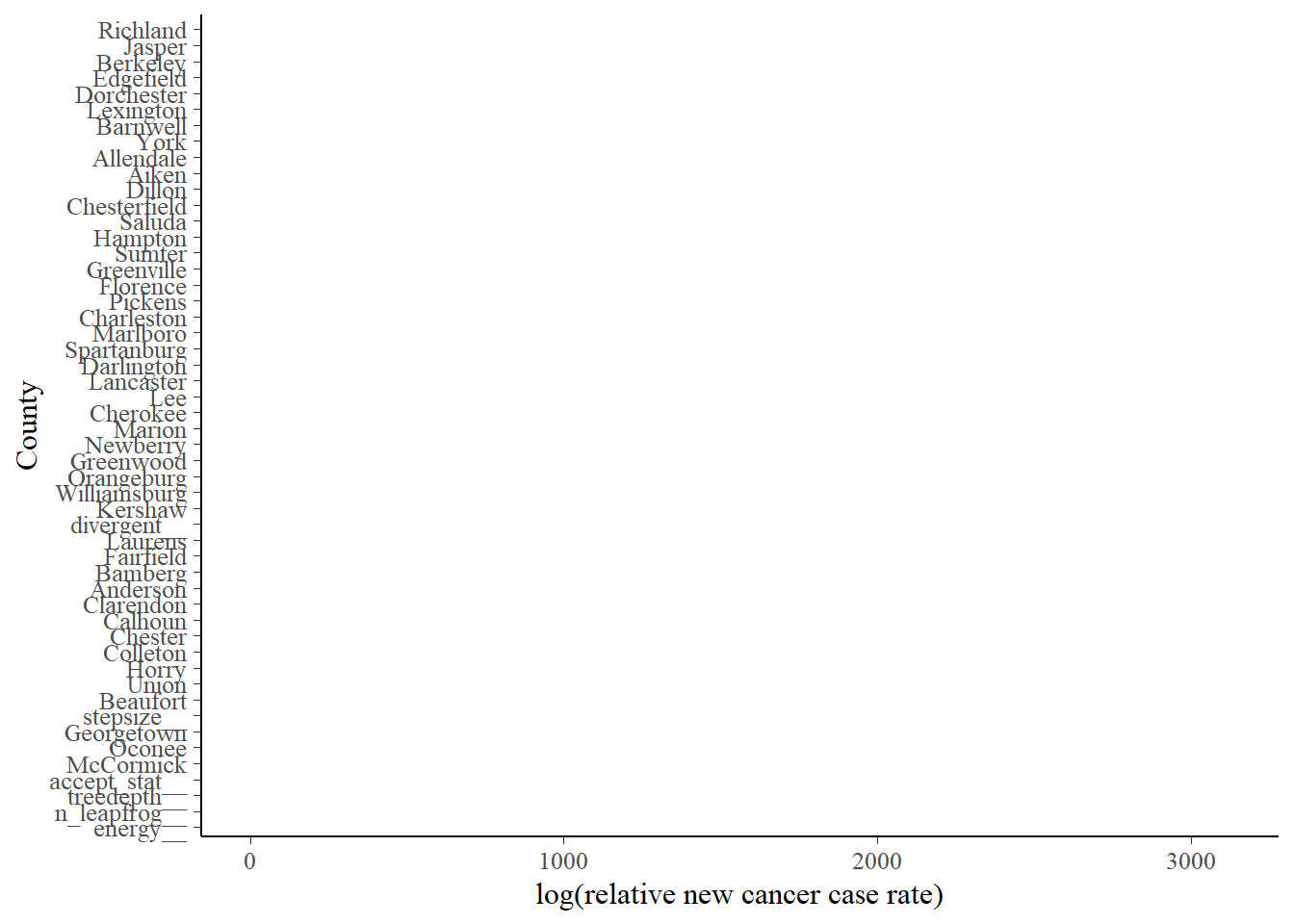
The forest plot version looks like this:
bayes_pois_fit %>%
  tidy_draws() %>%
  gather(variable, draw, 4:ncol(.)) %>%
  filter(variable %nin% c("year_mod", "(Intercept)")) %>%
  ggplot(aes(x = draw, y = fct_reorder(variable, draw, .desc = TRUE))) +
  stat_pointintervalh(.width = c(0.8, 0.95)) +
  scale_y_discrete(labels = function(.x) str_remove(.x,"county")) +
ylab("County") + xlab("log(relative new cancer case rate)") 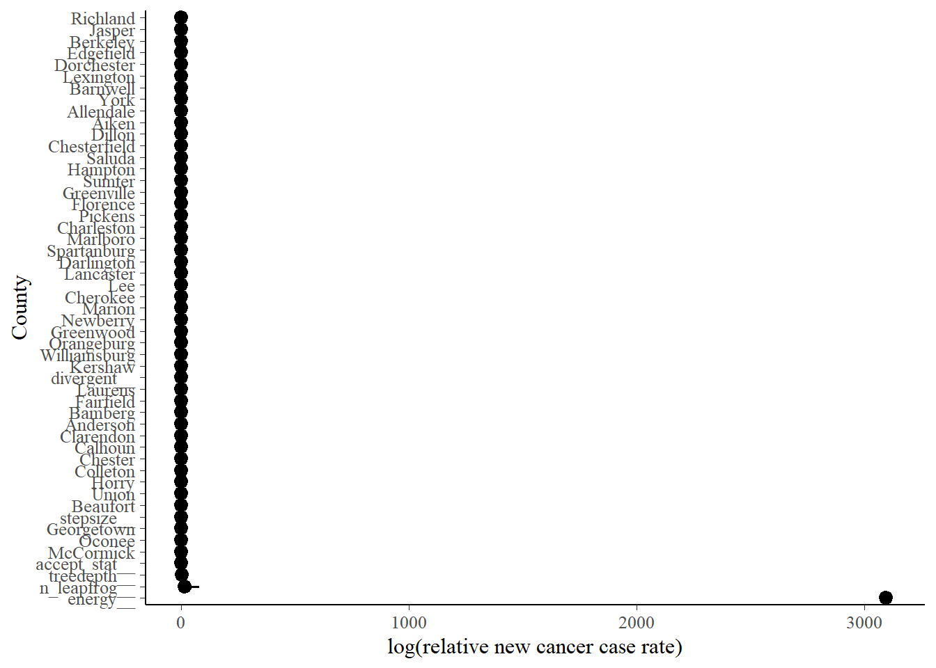
There’s a couple of neat tricks used above to easily pretty up this graph. First, the variable names for the counties come out of the analysis looking like countyMcCormick, for example. We clean that up using the str_remove function from the stringr package inside of scale_y_discrete. We are then left with the raw county names to appear on the tick marks. Another is using %nin% (that strange function I defined way above instead of loading all of Hmisc) inside of the filter function to select just the county variables. You may or may not have to get more clever when you do your own analysis, or you might use the functionality inside of spread_draws or gather_draws. Finally, I used fct_reorder inside of the aes function in ggplot above to reorder the counties in a meaningful way for interpretation. If your plot looks like an uninterpretable jumble, give that function a look; it’s part of the forcats package loaded by tidyverse.
So, for interpretation: if we look a the bottom of the graph we find Georgetown, Oconee, and McCormick counties, which we saw when we looked at the worst counties. At the top, we see Richland and Jasper, which matches our exploratory analysis above. Oconee is way out of the way with no heavy industry that I know of, so it’s pretty curious it’s showing some of the highest rates.
Conclusion
Well, that does it for this introduction. I want to take a deeper dive into tidybayes next time using this same dataset and model. We accomplished a lot in this post:
- Downloaded and processed data on new cancer rates in SC
- Scraped the statistical abstract website of SC for population estimates from the census
- “Mashed up” the two datasets
- Some exploratory analysis
- Formulated a rather sophisticated model using the
rstanarmpackage - Presented some results, compared them back to the exploratory analysis, and provided some interpretation
- As a bonus, created a function that really should have been a part of base R to begin with