Analyzing GSP flights using Bayesian analysis with Stan
Introduction and purpose
This is a new series on Bayesian analysis using Stan, and, specifically, the R interface to Stan. Even if you don’t want to use the R interface to Stan, much of the actual Stan code may still apply to you, but for now you are on your own getting data into and back out.
Bayesian analysis can be described in several different ways, all of which offer useful ways of thinking about problems. It requires a little bit of a paradigm shift if you are used to classical statistics or machine learning. For one thing, everything is assumed to be described by a random variable. For instance, if you are analyzing the height of all women in the world, we assume the height of any individual is random, but we also assume that the population average (a “parameter” or “unknown quantity” we might be trying to “estimate”) is also random. (Some frameworks, including classical statistics, would assume it fixed but ultimately unknowable.) The purpose of this series is to get some hands-on experience with Bayesian analysis and bring some of these theoretical ideas more concrete, so they can be used for practical, real-world cases.
We’ll start simple and work our way to more complex cases over time. During this series, we’ll encounter some philosophical struggles, some more practical matters, and some computing issues that will make us try different approaches.
One note: you can get help on rstan by using help("rstan") once you’ve loaded the package. For some reason, they seem to use partial pooling as the simplest example, and while partial pooling is important, it might be a little confusing while you are getting started. I get a lot simpler here.
In a previous post, I analyzed the number of departing flights from the local Upstate airport GSP (Greenville-Spartanburg International). There were some interesting patterns in the data. I think it will serve as an interesting launch point for a new series on using the Stan package for Bayesian analysis.
Installation
First, you’ll need to install R, if you don’t have it. Head over to http://www.r-project.org if you don’t. I also install the Rstudio (http://www.rstudio.com) IDE for R, because it has a lot of nice features (including integrating R code in blogging!).
Once you have R, you will need to install the rstan package. (While you’re at it, pick up the rstanarm package as well, for later on.) For readability of data manipulation, I’ll use dplyr and related packages (collectively known as the “tidyverse”). Use install.packages(c("rstan","rstanarm","tidyverse","lubridate")) to get these packages; all relevant dependencies will be installed. (I also use the lubridate package to manage some of the strange date formats – I understand it will be included in tidyverse at a later date). For more information on the tidyverse packages, go over to http://tidyverse.org, but after you’ve finished reading about Stan here :).
And now we begin.
Setup and data
First we load our packages.
library(tidyverse)
library(lubridate)
library(rstan)
The tidyverse package will load a number of packages, including dplyr and lubridate. dplyr is a very nice package which performs data manipulation in an intuitive fashion, including the use of the pipe %>% operator which you will see in action. I turned off the rather verbose messages for the purposes of blogging, but if you are familiar with R you may want to review them for some gotchas.
One thing you notice as you load rstan is the following:
Loading required package: StanHeaders
rstan (Version 2.17.2, GitRev: 2e1f913d3ca3)
For execution on a local, multicore CPU with excess RAM we recommend calling
options(mc.cores = parallel::detectCores()).
To avoid recompilation of unchanged Stan programs, we recommend calling
rstan_options(auto_write = TRUE)

Attaching package: 'rstan'
Chances are, you have at least a dual core machine, and you really don’t want to compile every time you run. So run the suggested code:
options(mc.cores = parallel::detectCores())
rstan_options(auto_write = TRUE)
Now, as before, I load the data:
load("airline_data.RData")
airline_data %>%
  mutate(date=ymd(YEAR*10000+MONTH*100+DAY_OF_MONTH),
         wnum = floor((date - ymd(YEAR*10000+0101))/7)) ->
  airline_data

airline_data %>%
  filter(ORIGIN_AIRPORT_ID==11996) %>%
  count(date) ->
  counts_depart

counts_depart %>%
  ggplot(aes(date,n)) +
  geom_line() +
  scale_x_date(date_breaks = "1 month", date_labels = "%b %y") +
  ylab("Number of departing flights") +
  xlab("")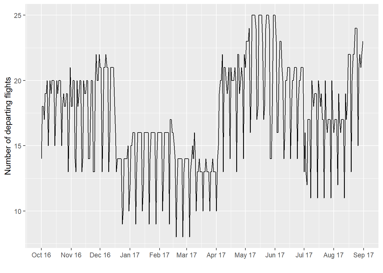
This code, as before, loads the airline data and converts the rather strange date format to a date format that R can use. (See the linked post for more details – I more or less copied the first part of the code.) I then display the counts again just to show what we’re working with. (Again, to obtain the original csv data, refer to the linked post.)
Simple model of how many flights per day
So, to start, we will start with a very simple model of the number of flights per day: a mean plus some noise. If this rankles because of the rich structure you saw in the plot above, well that’s a good sign but for now you can be patient. This post is part of a series, after all, and we’ll get to all that. But for now, we’re introducing Stan and progressing from simple to more complex models. This is a path you might take with other examples, after all.
Modeling the data
So the model is
\[\textrm{flights per day} \sim \scr{N}(\mu,\sigma)\] where \(\scr{N}\) is the normal distribution, \(\mu\) is some average number of flights, and \(\sigma\) is the standard deviation of some random noise. Basically, the model states we have the same number of flights every day, with the exception of some random variation. The higher the \(\sigma\), the higher the variation.
This model’s not “actually true,” but it will serve as a starting point. (If you’re scared of the math symbols, hang in there, I’ll keep you posted on what they mean.)
One of the joys of Stan is that this equation translates directly into a model:
parameters {
  real mu;
  real<lower=0> sigma;
}

model {
  flights ~ normal(mu,sigma);
}
If you’re into statistics, you might read the ~ as “is distributed as”. In addition, you might have noticed a strange <lower=0> for sigma. That’s because we don’t want our standard deviation to go below 0. That would just make no sense at all.
In fact, the Stan code is nearly written by the above. We have two things left to do:
- add a prior distribution to
mu, which reflects our current belief about the number of flights departing from GSP, and - connect the data with the model through the
flightsvariable.
Adding the prior distribution of mu and sigma
We add the prior distributions on mu and sigma. As mentioned above, everything is random, and these parameters are no different. We characterize our “prior belief” about these parameters with a probability distribution.
GSP has 13 gates, and about 8 or so seem to be busy (for GSP). Let’s say we observe a gate doing about 4 flights a day, so we might guess that GSP sends out 32 flights a day. But we’re really taking a stab in the dark here, so we’re not sure. So we put a standard deviation of 10 around this 32. So we would state the prior distribution as follows:
\[\mu \sim \scr{N}(32,10)\]
Furthermore, we have no idea what the standard deviation of the number of flights is, so we might use a uniform prior. The term “uniform” means that we will place equal belief in all parameters in a particular range. So, if we put a prior uniform between 0 and 20 on \(\sigma\), we are stating we believe the standard deviation is somewhere between 0 and 20, but we really don’t have any better information at this point. The hope is that this uniform prior will let the data speak for itself.
\[\sigma \sim \textrm{Uniform}(0,20)\]
This is reflected in the model statement in Stan, pretty much the way you see it above.
parameters {
  real mu;
  real<lower=0> sigma;
}

model {
  flights ~ normal(mu,sigma);
  mu ~ normal(32,10);
  sigma ~ uniform(0,20);
}
Connecting the data to the model
So there are three things in the model block above: mu, sigma, and flights. Flights, as you might expect, reflect our data. To make this connection, we have to tell Stan that it should expect flights as a data source. Thus, we add a data block to the Stan code above.
There is one minor detail. It’s really helpful to pass in the number of observations as well so we can tell Stan how much data there is. There’s one strange caveat: I had to define flights as a real vector and not a vector of integers. This is because I put a normal distribution on it. We’ll consider alternatives later.
data {
  int ndates;
  vector[ndates] flights;
}

parameters {
  real mu;
  real<lower=0> sigma;
}

model {
  flights ~ normal(mu,sigma);
  mu ~ normal(32,10);
  sigma ~ uniform(0,20);
}
That’s it for the Stan code! We can package this up and put it in a .stan file and use it. Note if you’re using RStudio, it understands .stan files and will apply helpful syntax highlighting. I’ve done this and called the program flights.stan.
Passing data to the model
All that remains is to glue the data and the model together. Our data was created above and is stored in counts_depart. For purposes here, all we need are the number of rows, which will pass to ndates in the Stan model, and the number of flights. (Hold on there grasshopper! We’ll use the dates later in the series.)
This is done in two steps:
- Defining variables holding our data that match up with what we defined in the
.stanfile (so,ndatesandflightsfound in thedatablock) - Calling Stan using the
stanfunction from therstanpackage and telling it what data you want to pass
So let’s do it. Go back to your favorite R editor and key it in:
ndates <- nrow(counts_depart)
flights <- counts_depart$n

data_to_pass <- c("ndates","flights")
mean_model_fit <- stan("flights.stan",data=data_to_pass)
save(mean_model_fit,file="mean_model_fit.RData")
This last save step is so we can re-use the mean_model_fit file later.
Results
The first time you run the .stan file, it has to compile. The developers have some magic where they turn Stan code into C++. The upshot is that the first run takes longer than subsequent runs. But, if you wanted to change the data and run it again, it can skip the compiling and go straight to the running. Of course, if you change the model, Stan has to recompile. With that caveat out of the way, let’s see what the fit looks like.
mean_model_fit## Inference for Stan model: flights.
## 4 chains, each with iter=2000; warmup=1000; thin=1;
## post-warmup draws per chain=1000, total post-warmup draws=4000.
##
## mean se_mean sd 2.5% 25% 50% 75% 97.5% n_eff
## mu 17.33 0.00 0.21 16.92 17.18 17.33 17.47 17.73 3831
## sigma 3.91 0.00 0.16 3.61 3.80 3.90 4.01 4.22 3732
## lp__ -623.15 0.02 1.00 -625.81 -623.54 -622.85 -622.44 -622.17 1931
## Rhat
## mu 1
## sigma 1
## lp__ 1
##
## Samples were drawn using NUTS(diag_e) at Tue Jan 08 16:27:56 2019.
## For each parameter, n_eff is a crude measure of effective sample size,
## and Rhat is the potential scale reduction factor on split chains (at
## convergence, Rhat=1).First thing we want to look at is to make sure Stan did ok with the model. We didn’t see any funny error messages above (just some warnings in the compile stage that we can ignore). We also want to look at the Rhat - if it’s around 1, then we’re generally ok. The n_eff variable should also be fairly high - fully efficient would be the # of post-warmup draws (here 1000) times the number of chains (here 4). Because n_eff compares favorably to 4000, we can have some more confidence. We’ll ignore the lp__ (stands for log posterior) for now and revisit it later. This was a fairly simple model, so we would expect Stan to do fine.
Here, our model shows that there is an average of around 17.33 flights per day - mu above as a mean of 17.33. The standard deviation is around 3.91. Because mu is a random number (recall our Bayesian philosophy above that everything is random), it could vary, and the percentiles above give us an idea of about how much. It has a 2.5% chance of being 16.90 or below and a 2.5% chance of being above 17.75.
Notice that our original back-of-the-envelope estimate of 32 was way off, but we also expressed a lack of confidence by putting a high standard deviation on our prior. Here, we say “the data overwhelmed the prior”. We might rethink how we came up with that estimate - recall we had taken some guesses about the number of gates in operation and number of flights from those gates. Maybe we were wrong in one or both of those assumptions.
Our standard deviation is also pretty high - if we do a back-of-the-envelope calculation of number of flights on any given day, there’s a 95% chance (or so) that it will be between 17.33 - 2 x 3.91 (so, a bit above 9) and 17.33 + 2 x 3.91 (so, around 25). The graph above suggests more is going on, such as differences based on weekday or season.
Discussion
Here we really dipped our toes into Stan with a very simple model. We talked about how to go from math to Stan code, which I personally think is the power of Stan. Specifically, you can make the transcription very easy in the model block. Then we talked about how to connect our data to the model using the rstan package. Then we did a little assessment of our model and looked briefly at the results.
We’re just getting started, and there are a lot of ways we can extend this example, and I will get to many of these topics in later posts:
- More analysis of output
- Better models (models of counts, seasonality, correlation, analysis of variance)
- Things that can go wrong with a Stan fit (divergent transitions and funnels, oh my!)